A Random Walker Based Approach to Combining Multiple Segmentations .... arg max. ËS Ï(ANMI)(ËS,Î) where ËS covers all possible K â [Kmin,Kmax] seg-.
A Random Walker Based Approach to Combining Multiple Segmentations P. Wattuya, K. Rothaus, J.-S. Praßni, and X. Jiang Department of Computer Science, University of M¨unster, Germany {wattuya,rothaus,j pras01,xjiang}@math.uni-muenster.de Abstract In this paper we propose an algorithm for combining multiple image segmentations to achieve a final improved segmentation. In contrast to previous works we consider the most general class of segmentation combination, i.e. each input segmentation has an arbitrary number of regions. Our approach is based on a random walker segmentation algorithm which is able to provide high-quality segmentation starting from manually specified seeds. We automatically generate such seeds from an input segmentation ensemble. An informationtheoretic optimality criterion is proposed to automatically determine the final number of regions. The experimental results on 300 images with manual ground truth segmentation clearly show the effectiveness of our combination approach.
1
Introduction
Despite of decades of intensive research unsupervised image segmentation remains a difficult task. Recently, researchers start to investigate combination of multiple segmentations. Several works in medical image analysis consider segmenting an image into a known number of semantic labels [8]. Typically, such algorithms are based on local (i.e. pixel-wise) decision fusion schemes such as voting. Alternatively, a shapebased averaging is proposed in [7] to combine multiple segmentations. The works [4, 5] deal with the general segmentation problem. However, they still assume that all input segmentations contain the same number of regions. In [4] a greedy algorithm finds the matching between the regions from the input segmentations which build the basis for the combination. The authors of [5] consider an image segmentation as a clustering of pixels and apply a standard clustering combination algorithm for the segmentation combination purpose. Our work is not limited to this restriction and we consider the most general case (an arbitrary number of regions per image). The work [9] makes clever use of multiple segmentations to automatically discover objects in a variety of image datasets. However, no multiple segmentation combina-
978-1-4244-2175-6/08/$25.00 ©2008 IEEE
tion is presented in this work. An ensemble Λ = {S1 , ..., SN } of N segmentations of the same image can be produced by using different algorithms or with the same algorithm but different parameter values. Our goal is to compute a final segmentation result which is superior to the initial segmentations in a statistical sense (to be specified later). We continue with a brief discussion about the need of segmentation combination to motivate our work. Then, our random walker based approach is presented in Section 3. An optimality criterion for automatically determining the region number K is proposed in Section 4. Experimental validation is reported in Section 5, followed by some discussions to conclude this paper.
2
Need of Segmentation Combination
Segmentation algorithms mostly have some parameters and their optimal setting is a non-trivial task. We propose to implicitly explore the parameter space (without the need of ground truth segmentation). A reasonable parameter subspace (i.e. a lower and upper bound for each parameter) is assumed to be known and is sampled into a finite number N of parameter settings. Then, we run the segmentation procedure for all these N parameter settings and compute a final combined segmentation of the N segmentations. The rationale behind our approach is that this segmentation tends to be a good one within the explored parameter subspace. In addition it is possible to combine the results of different segmenters to benefit from their strengths. Similarly, we may compute a single representative from multiple manually specified ground truth segmentations. In all these application scenarios we need a robust combination algorithm.
3
The Algorithm
The basis of our multiple segmentation combination algorithm is the random walker algorithm for image segmentation [2]: Given a small number of K seeds (groups of pixels with user-defined labels), the algorithm labels unseeded pixels by resolving the probability that a random walker starting from each unseeded
pixel will first reach each of the seeds. A final segmentation is derived by selecting for each unseeded pixel the most probable seed destination for the random walker. The algorithm can produce a quality segmentation provided suitable seeds are placed manually. The random walker algorithm is formulated on an undirected graph G = (V, E, w), where each pixel pi has a corresponding node vi ∈ V . Each edge eij ∈ E has a weight wij indicating similarity between the neighboring pixels vi and vj (in 4-neighborhood). Given such a graph and the seeds, the probability of all unseeded pixels reaching the seeds can be efficiently solved. There exists a natural link of our problem at hand to the random walker based image segmentation. The input segmentations provide strong hints about where to automatically place some seeds. Given such seed regions we are then faced with the same situation as image segmentation with manually specified seeds and can thus apply the random walker algorithm [2] to achieve a quality final segmentation. To develop a segmentation ensemble combination algorithm based on the random walker we need three components: Generating a graph to work with (Section 3.1), extracting seed regions (Section 3.2) and computing a final combined segmentation result (Section 3.3).
3.1
Graph Generation
In our context the weight wij should indicate how probably the two pixels pi and pj belong to the same image region. Clearly, this can be guided by counting the number nij of initial segmentations, in which pi and pj share the same region label. Thus, we define the weight function as a Gaussian weighting (in accordance with [2]): wij = exp (−β · (1 −
nij )) N
where β is a free parameter of the algorithm. Low edge weights indicate high probabilities of region boundary evidence between two neighboring pixels and avoid a random walker crossing these boundaries.
3.2
Seed Region Generation
We describe a two-step strategy to automatically generate seed points: (i) extracting candidate seed regions from G; (ii) grouping them to form final seed regions to be used in the combination step. Candidate seed region extraction: We build a new graph G∗ by preserving those edges with weight wij = 1 only (pi and pj have the same label in all N initial segmentations) and removing all other edges. This step basically retains those edges between two neighboring
nodes (pixels) which are most likely to belong to the same region. Then, we detect all connected subgraphs in G∗ and regard them as a set of initial seed regions which are further reduced in the next step. Grouping candidate seed regions: The number of candidate seed regions from the last step is typically higher than the true number of regions in an input image. Thus, a further reduction is performed by iteratively merging the two closest candidate seed regions until some termination criterion is satisfied. For this purpose we need a similarity measure s(Ci , Cj ) between two candidate seed regions Ci and Cj and a termination criterion. For pi ∈ Ci and pj ∈ Cj , nij /N clearly provides a hint of the similarity s(Ci , Cj ) at the individual pixel level. At the global level we thus define s(Ci , Cj ) by the average of all such pixel pairs: s(Ci , Cj ) = {nij /N | (pi , pj ) ∈ Ci × Cj }
(1)
where A denotes the average of the set A. We iteratively select two candidate seed regions with the highest similarity value and merge them to build one single (possibly spatially disconnected) candidate seed region. Then, the similarity values between a new merged region and all remaining candidate seed regions are recomputed. The operation is stopped if the highest similarity is below a threshold tregion , which indirectly determines the number of seed regions K. Another strategy without using the threshold tregion is to generate a series of results with K ∈ [Kmin , Kmax ] seed regions. Then, each initial result is fed to the ensemble combination part of our algorithm (Section 3.3) to achieve Kmax −Kmin +1 combination segmentations and we select an optimal one as the final combination segmentation (Section 4). Implementation details: Computing Eq. (1) can be quite time-consuming for large images. In practice, using only a small fraction of pixels per region is sufficient to estimate the similarity measure. We thus randomly select ten pixels per region for the similarity computation. Furthermore, only the first 50 largest candidate seed regions are used in the merging process. This number is experimentally determined to be large enough to cover all salient natural image segments. These two details improve the computational efficiency of our algorithm without degrading the combination quality.
3.3 Segmentation Ensemble Combination Given the graph G constructed from the initial segmentations and K seed regions, we apply the random walker algorithm [2] to compute the combination segmentation. The computation of random walker probabilities can be exactly performed without the simulation
of random walks, but by solving a sparse, symmetric, positive-definite system of equations. Each unseeded pixel is then assigned a K-tuple vector, specifying the probability that a random walker starting from that pixel will first reach each of the K seed regions. A final segmentation is derived by assigning each pixel the label of the largest probability.
4 Optimization of K In general the true number of regions K is unknown. When computing a series of combination segmentations with K ∈ [Kmin , Kmax ] seed regions, we need a way of selecting the optimal one. The quality of combination results can be evaluated in terms of consistency with the input ensemble. A good combination should share as much information as possible with the given N segmentations. We follow the concept of mutual information to quantify the statistical information shared between two segmentations. An optimality criterion is proposed to determine the optimal K. We define the normalized mutual information φ(NMI) between two segmentations Sa and Sb by |Sa | |Sb | � �
|Rh,l | log
n · |Rh,l | |Rh | · |Rl |
φ(NMI) (Sa , Sb ) = � h=1 l=1 � |Sa | |Sb | �� |Rh | � |Rl | � |Rh | log |Rl | log n n h=1
l=1
where Rh and Rl are regions from Sa and Sb , respectively, Rh,l denotes the common part of Rh and Rl , and n is the image size. The value domain of φ(NMI) is [0, 1]. Then, an information-share measure between a single segmentation Sˆ and a set Λ = {S1 , . . . , SN } of N input segmentations can be defined as the average normalized mutual information (ANMI): N � ˆ Λ) = 1 ˆ Sq ) φ(NMI) (S, φ(ANMI) (S, N q=1
We propose to select the optimal combination segmentation S kopt as the one with maximal average mutual information among all individual segmentation Sq in Λ: ˆ Λ) S kopt = arg max φ(ANMI) (S, ˆ S
where Sˆ covers all possible K ∈ [Kmin , Kmax ] segmentations. If we replace Sˆ by a universe U of all possible segmentations of an image, then S kopt would represent the optimal segmentation in accordance with the generalized median concept of the input ensemble [3]. There-
fore, our approach can be regarded as an approximation of generalized median segmentation by investigating the subspace of U consisting of the combination segmentations for all possible K ∈ [Kmin , Kmax ] only.
5
Experimental Results
We tested our algorithm on 300 natural images of size 481 × 321 from the Berkeley segmentation dataset [6], each having multiple manual segmentations. We apply φ(NMI) to quantitatively evaluate the segmentation quality against the ground truth. One segmentation result is compared to all manual segmentations and the ANMI is reported. Larger ANMI values indicate better combination results that share more information with the ground truths. The graph-based image segmentation algorithm [1] was used as the baseline segmentation method. This decision was made because of its competitive segmentation performance and high computational efficiency. The algorithm has three parameters: smoothing parameter (σ), a threshold function (k), and a minimum component size (min area). We obtained 24 segmentations of an image by varying the parameter values (fixing min area = 1500 and varying σ = 0.4, 0.5, 0.6, 0.7, 0.8, 0.9 and k = 150, 300, 500, 700). We empirically set the parameters β and tregion (for the version without automatic determination of K) to 30 and 0.7, respectively, for all experiments. The proposed algorithm was implemented in MatLab on an Intel Core 2 CPU. Seed region extraction (Section 3.2) for an image requires 1 second in average and less than 2 seconds are needed for the random walker algorithm for the final combination step (Section 3.3). Figure 1 shows two examples of combined segmentations produced by our method: (d) without the optimality criterion (using a threshold tregion to determine K), (e) automatic determination of K. For comparison purpose we also show the input segmentation with the worst, median and the best ANMI values ((a)-(c)). Generally, we can observe a substantial improvement of our combination compared to the median input segmentation. These results demonstrate that we can obtain an “average” segmentation which is superior to the - possibly vast - majority of the input ensemble. Indeed, this behavior can be systematically validated on the entire database of 300 images. Figure 2 shows the average performance of all 300 images with regard to each of the 24 individual configurations (parameter settings). Figure 1 (e) shows the combination result with optimization of K obtained by running the combination algorithm multiple times, varying the region number K in an interval [2, 50] and then selecting the combination result with the greatest ANMI. The results demonstrate
80
0.62
70
0.61
60
0.6
50
(a) ANMI = 0.6083
(b) ANMI = 0.6577
(c) ANMI = 0.6997
images
ANMI
0.59 0.58
20
0.56 0.55
Combined results without optimizing K Combined results with optimal K the average performance of each individual parameter setting
0.54 0 1 2 3 4 5 6 7 8 9 10 11 12 13 14 15 16 17 18 19 20 21 22 23 24 Parameter setting
(a) (d) k=21; ANMI=0.7102 (e) k=20; ANMI=0.7172
(a) ANMI = 0.5771
(b) ANMI = 0.7026
40 30
0.57
10 0
0 1 2 3 4 5 6 7 8 9 10 11 12 13 14 15 16 17 18 19 20 21 22 23 24
(b)
Figure 2. (a) Average performance of combined results over 300 images for each individual parameter setting. (b) f (n): Number of images for which the combination result is worse than the best n input segmentations. (c) ANMI = 0.8069
(d) k=10; ANMI=0.7722 (e) k=7; ANMI=0.8141
Figure 1. (a)-(c) show three input segmentations with the worst, median and the best ANMI, respectively. (d) Combined segmentation of the proposed algorithm and (e) Combined segmentation with optimal K.
values and selecting an optimal segmentation based on an information-theoretic optimality measure. A robust segmentation combination algorithm provides the basis for several ideas outlined in Section 2 to alleviate some hard problems in image segmentation. The current work represents a first step towards that development. Other future work includes an extension of our approach to other problem domains.
References the effectiveness of the optimality criterion. We can achieve an improvement of combination result (more close to the ground truth). In many cases we can even achieve some improvement against the best input segmentation. The red line in Figure 2 (a) demonstrates the average performance of this automatic determination of K against the average of all 300 images. Figure 2 (b) shows a histogram f (n), indicating the number of images among the 300 test images, for which the combination segmentation is worse than the n best input segmentations. Remarkably, the combination segmentation outperforms all 24 input segmentations in 78 cases, including the two examples in Figure 1. For 70% (210) of all 300 test images, the goodness of our solution is beaten by at most 5 input segmentations only. This statistic is a clear sign of combination quality of our approach.
6
Conclusion
In this work we have taken some steps towards a framework of multiple image segmentation combination based on the random walker idea. In contrast to the few early works we consider the most general class of segmentation combination, i.e. each input segmentation can have an arbitrary number of regions. Our algorithm is efficient enough to be capable of evaluating a series of possible combination results with different K
[1] P. Felzenszwalb and D. Huttenlocher. Efficient graphbased image segmentation. International Journal of Computer Vision, 59(2):167–181, 2004. [2] L. Grady. Random walks for image segmentation. IEEETPAMI, 28(11):1768–1783, 2006. [3] X. Jiang, A. M¨unger, and H. Bunke. On median graphs: Properties, algorithms, and applications. IEEE-TPAMI, 23(10):1144–1151, 2001. [4] Y. Jiang and Z.-H. Zhou. SOM ensemble-based image segmentation. Neural Processing Letters, 20(3):171– 178, 2004. [5] J. Keuchel and D. K¨uttel. Efficient combination of probabilistic sampling approximations for robust image segmentation. DAGM-Symposium, pages 41–50, 2006. [6] D. R. Martin, C. Fowlkes, D. Tal, and J. Malik. A database of human segmented natural images and its application to evaluating segmentation algorithms and measuring ecological statistics. ICCV, pages 416–425, 2001. [7] T. Rohlfing and C. R. Maurer Jr. Shape-based averaging for combination of multiple segmentations. MICCAI (2), pages 838–845, October 2005. [8] T. Rohlfing, D. B. Russakoff, and C. R. Maurer Jr. Performance-based classifier combination in atlas-based image segmentation using expectation-maximization parameter estimation. IEEE Trans. Med. Imaging, 23(8):983–994, 2004. [9] B. C. Russell, A. A. Efros, J. Sivic, W. T. Freeman, and A. Zisserman. Using multiple segmentations to discover objects and their extent in image collections. CVPR, pages 1605–1614, 2006.