system, and a single board computer (SBC) running VxWorks 21], a real-time operating system. In this kind of agile manufacturing system, the software plays a ...
1
A REAL-TIME DATABASE SERVER IN AN AGILE MANUFACTURING SYSTEM SungKil Lee, Huang-Cheng Kuo, N. Hurkan Balkir, YooHwan Kim, and Gultekin O zsoyo�glu
Department of Computer Engineering and Science Case Western Reserve University, Cleveland, Ohio 44106
ABSTRACT The term agile manufacturing refers to a manufacturing system that can fabricate various products simultaneously without long downtimes for retooling. Agile manufacturing systems can bene t signi cantly from a database support and more speci cally from real-time database systems. This chapter describes AMDS, an agile manufacturing database system designed for capturing and manipulating the operational data of a manufacturing cell. AMDS is a continuous data gathering, real-time DBMS, and it can be logged either locally or remotely and used for o�-line analysis as well. The temporal operational data obtained is used for performance and reliability analysis, high-level summary report generation, real-time monitoring and active interaction. This chapter describes the overview of AMDS, its real-time features and the cooperative transaction model that it employs.
1 INTRODUCTION In this chapter, we describe the case study of a real-time database system for a speci c kind of operational data generated by an agile manufacturing system. The term agile manufacturing refers to a manufacturing system that can fabricate various products simultaneously without long downtimes for retooling. The agile manufacturing increases competitiveness of companies in the market by decreasing the downtime and recon guration overhead incurred due to product changes. The agile manufacturing concept is already in a stage of practical 1
2
Chapter 1
use in some companies, for example, pager manufacturing at Motorola [19], or customized bicycles from Panasonic [5]. At Case Western Reserve University (CWRU), a testbed agile manufacturing system for light mechanical assembly has been developed [17]. The system is used for producing various kinds of plastic assemblies from the same workcell with minor changes to modular tables and robot grippers. Currently, the system uses a Bosch automation system, multiple Adept [2] robots and a vision system, and a single board computer (SBC) running VxWorks [21], a real-time operating system. In this kind of agile manufacturing system, the software plays a more important role than in a conventional manufacturing system. The software takes control of the work sequence and the product changeover. Our agile manufacturing software gathers operational data when running an agile manufacturing system, and stores the operational data that is generated during operation into a database system, called AMDS (Agile Manufacturing Data Base System). Such temporal data is used for the following activities.
(1) O�-line Analysis: (a) Performance Analysis: By statistically analyzing the operational
data, the performance of the system is evaluated critically. And, the performance variations due to improvements and modi cations to the workcell are quantitatively measured. (b) Reliability Analysis: Errors and disruptions that occur during operations are logged, and later analyzed through summary statistics. This leads to quantitative and measurable evaluations about how reliable each component of the workcell is. (c) High-Level Summary Reports: The productivity and activities of the workcell are summarized and reported. (2) Real-Time Monitoring: Critical operational data during execution are rerouted to operator terminals and displayed for observation and human intervention when necessary. Real-time operational information is provided for the development of workcell software and high-level decision making. The information is deduced from the available operational data stored in the database system. Such information is crucial in the development stage for reliability, fault-detection and analysis. (3) Active Interaction: Events of the Agile Manufacturing System are identi ed, classi ed, and, for di�erent events, di�erent database actions are
Real-Time Database In Agile Manufacturing
3
de ned as rules. A rule r is of the form \if the event E occurs and the condition C holds then take the database action A within time quota t". One example of a database action is to initiate a query for the throughput information of a certain robot in the last hour. Such rules form a rule-base and are changed any time the behavior of the system needs to be changed. By implementing an event-monitoring software and a rule manager software, rules are triggered and executed during the operation of the workcell. This makes the data management active in the sense that, at operation time, the Agile Manufacturing software takes actions as a response to event occurrences. It is also adaptive in the sense that rules are changed easily re ecting the changes to the actions of the system. The manufacturing workcell prototype at CWRU, called the Agile Manufacturing System (AMS), is currently functional. However, there still exist workcell stoppages and faulty operations. Two approaches are considered for operational errors: prevention and recovery. We use the cooperative transaction model [11] that we have developed to implement mechanisms for preventing potential errors and for fast recovery from these errors. For the prevention, the database system examines the operation condition upon the completion of a batch (a pallet) of assembly products. The database system receives a message from the manufacturing control system on the amount of assembled products and the tools used for manufacturing. If the accumulated amount of assembled products by a tool reaches the maintenance (or replacement) level of the tool, a maintenance (or replacement) order is generated. This can be done by applying the alerter mechanism of active database systems. For support in error recovery, when a manufacturing error occurs, the manufacturing control system identi es the error location, and queries the database system to get additional information to solve the problem. Database transactions communicate with each other to share fundamental information to locate the problem. Also, rule actions (which are also transactions) are triggered in order to coordinate necessary recovery steps. Rules for critical events and actions have high priorities. The rest of the chapter is organized as follows: In section 2, we discuss the agile manufacturing workcell system and user requirements. Section 3 presents the agile manufacturing database system. In sections 4 and 5, we discuss the design of the data model for the application database and integrity constraints. Section 6 discusses data logging techniques. In section 7, we present examples of real-time queries and rules. In section 8, conclusions and future work are presented.
4
Chapter 1
2 AGILE MANUFACTURING APPLICATION DOMAIN 2.1 Agile Manufacturing Workcell This section describes the workcell hardware and software which generates the operational data [17]. The basic structure of the workcell is composed of a central circular conveyor system, multiple Adept robots, modular worktables,
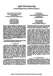
exible part feeders, and pallets to contain subassemblies. Parts are recognized by the Adept vision system through cameras mounted on the workcell frame. The workcell hardware is designed to be modular to accomodate changes in assembly products. Special purpose devices are placed on modular work tables for the jobs that robots cannot perform easily. Modular robot grippers are used to increase agility. (Depending on the current assembly product, a gripper can be replaced by another.) Feeders provide assembly parts to robots continuously. At the end of each feeder, there is a small lighted window on which parts are placed for a CCD camera to view. The image taken from the camera is translated into a black and white image in which the sillouette of the parts produces a black area in contrast to the white lighted background. The image is processed by the Adept vision system to produce a part location value. Once the location is known, the robot grabs the part and either puts it on a worktable or assembles it with another part. Once a subassembly is made by a robot, it is placed on a pallet, and this cycle continues until a pallet is lled. A pallet with subassemblies is delivered to the next robot by the conveyor system. A pallet is a thin and solid plastic piece which is used for carrying subassemblies and delivering them to the next assembly station. Figure 1 shows the bill of material for light mechanical assembly of a telephone receiver. A telephone receiver has the following components: a handle (Handle), a receiver unit (Rec Unit), a receiver cap (Rec Cap), a cotton ball (Cot Ball), a transmitter cap (Tran Cap), a transmitter unit (Tran Unit), a transmitter holder (Tran Hold), and a socket (Socket) for the cord from the telephone base. The workcell software of AMS is designed for rapid changeover. The requirement for future maintenance is much greater than normal software projects due to the nature of agile manufacturing. The software design and implementation method currently used is object-oriented analysis and design. The goal is to con ne any design changes into a small area and to make the rest of the system una�ected, as well as making the tasks of adding or removing a part straightforward. For that, we need to separate variable parts in the workcell from xed parts.
Real-Time Database In Agile Manufacturing
5
Assembled_part Subass4 Subass3 Subass2 Subass1 Socket
Figure 1
Subass7
Tran_Cap Rec_Cap
Tran_Unit
Subass6
Cot_Ball
Rec_Unit
Handle
Tran_Hold
Bill of Material for Light Mechanical Assembly.
In addition to low-level hardware devices, we have also modeled the agents which are anticipated in any kind of manufacturing systems. The key to the agile software system is keeping the interface stable and each change strictly inside an object. For example, when the type of robot is changed, the assembler still has the same robot object and the interface. The system is implemented using C++ on VxWorks. The software program runs multiple tasks for controlling workcell devices such as conveyors, feeders, robots, vision system. There is also a task responsible for online data shipping over a 155 Mbits/sec ATM network to the AMDS database management system which runs on a separate workstation site. The robot motion command and vision command are performed by Adept's MV controller [1].
2.2 User Requirements We now identify the agile manufacturing database system objectives and specifically state what the agile database system does. These objectives are actually the requirements that users impose on the agile database system. Users perform the following activities.
{ On-line, real-time response to operator queries - canned or uncanned. The
agile database system provides SQL and relational algebra as its query language, through which the user is able to issue high-level commands or statements (such as SELECT, INSERT, etc)
Chapter 1
6
{ Periodic on-line queries for monitor views (summary data or actual data). { Actions (transactions) as responses to events (triggers/alerters/etc). { Data-processing reports. Reports are produced for job description, robot description, pallet description, part information, performance evaluation of robot, assembly information, product information, pallet location information, worktable description, robot activity information. Reports are used to 1. get speci c information such as the number of subassemblies generated by Robot1 and the number of assembly parts used by Robot2 , 2. diagnose the performance of workcell devices such as robots, feeders, vision, pallets, 3. maintain the assembly parts in workcell, 4. improve the development of workcell software, 5. prevent potential errors, and so on. We determine how often the real-time queries need to be evaluated (i.e., the periodicity), how fast the system must respond, what data is needed and in what format, and roughly how much data is involved. Figure 2 shows an example of a report that the agile database system generates and a statement of the requirements implied by this report. We will not be dealing with the issue of reports in this paper.
3 THE AGILE MANUFACTURING DATABASE SYSTEM (AMDS) AMDS is a relational prototype database system that handles real-time as well as non-real-time transactions and queries. AMDS receives a request from the AMS (agile manufacturing system) and returns the relevant information to the AMS. The operational data generated by AMS workcell software is stored into the database using either the bulk loader or the incremental loader. Bulk loader
Real-Time Database In Agile Manufacturing
Rob_id
Assem_action
Gripper_type
7
Raw_part_name Assem_part_name
Curly
Put_Handle
Handle_Gripper
Handle
Subass1
Curly
Put_Tran_Hold
Tran_Hold_Gripper
Tran_Hold
Subass1
Curly
Put_Ter_Screw
Ter_Screw_Gripper
Ter_Screw
Subass2
Curly
Move_sibass2
Handle_Gripper
Null_Part
Subass2
Larry
Put_Tran_Unit
Tran_Unit_Gripper
Tran_Unit
Subass3
Larry
Put_Tran_Cap
Tran_Cap_Gripper
Tran_Cap
Subass4
Larry
Mov_Subass4
Handle_Gripper
Null_Part
Subass4
Moe
Unload
Handle_Gripper
Null_Part
Subass4
Subass1=Handle + Tran_Hold
Subass2=Subass1 + Ter_Screw
Subass3=Subass2 + Tran_Unit
Subass4=Subass3 + Tran_Cap
a. Job Description Report Requirement: Robot Identification(Rob_id), Assembly Action (Assem_action),
Gripper Type (Gripper_type)
Raw Part Name (Raw_part_name), Assembly Part Name (Assem_part_name) How Often:
Once every 30 minutes
How Fast:
One minute b. Requirements Statement
Figure 2
Report and Requirements Statement.
stores previously collected operational data into the AMDS les, by parsing the conceptual model update operators of AMDS. Incremental loader, when activated, stores AMS operational data received by the Communication Interface. The Communication Interface (CI) is responsible for (a) receiving from the AMS Workcell Software (i) requests to load operational data into the Distributed-CASE-DB database, directed to the Bulk or the Incremental Loaders, (ii) requests to execute real-time relational algebra queries for DistributedCASE-DB to execute (for error recovery), (iii) requests to execute real-time transactions by the Coop-CASE-DB (for error recovery or panic operations). (b) receiving from the operators of the AMS Workcell Software (i) real-time relational algebra queries for Distributed-CASE-DB to execute. The queries are ad hoc, and are for error recovery, exploratory search and/or status checking.
8
Chapter 1
(ii) requests to execute real-time transactions by the Coop-CASE-DB (to check status, to produce reports, and/or to evaluate errors), (c) returning the responses to the requests of the AMS Workcell Software and the operators of the AMS Workcell. The responses are returned either as a single response or in multiple steps (through a simple browser), (d) displaying the output of periodic queries (for status reporting) on user monitors. User monitors are similar to those commonly found on factory
oors, and simply display the status of the AMS workcell. The Communication Interface communicates with the local processes using the UNIX Sysem V IPC primitives of shared memory and semaphores. The Communication Interface communicates with remote entities (i.e., the AMS Workcell Software, the AMS Workcell Operators and the user monitors) using TCP/IP Berkeley sockets [18]. The Coop-CASE-DB (which uses the cooperative transaction model and includes an event manager, a rule manager and a transaction manager) coordinates transaction execution to control time-critical manufacturing operations through a set of rules. The event manager detects manufacturing operation events and database operation events, and sends them to the rule manager. The rule manager periodically processes the events detected by the event manager and res rules. Transactions of red rules are scheduled for execution by the transaction manager. The communication between the client and the server is performed by the Communication Interface. Figure 3 shows the agile database server and its interaction with the agile manufacturing system. Distributed-CASE-DB [10, 16, 13] receives queries (time-constrained relational algebra expressions) issued by endusers to access the data, and parses and evaluates queries (operations), and returns the information to the enduser. AMDS contains a graphical query language, called VISUAL, that allows users to specify real-time, ad hoc, graphical queries. VISUAL can specify relational (and/or object-oriented) queires by diplaying icons of entities (i.e., relations in the relational model) and relationships (i.e., relations). VISUAL queries are translated into real-time relational algebra queries, and executed by Distributed-CASE-DB. Next we discuss the three main components of the AMDS, namely, the DistributedCASE-DB, the Coop-CASE-DB, and VISUAL.
Real-Time Database In Agile Manufacturing
User Monitor 1
User Monitor k
9
AMS Workcell Software
. . . Operator 1 Communication Interface (CI)
. . Operator m
Site 1
Coop-CASE-DB Event Manager
DistributedCASE-DB
Bulk Loader
Incremental Loader
. . Site n
Rule Manager Transaction Manager
VISUAL Transcation T1
AMDB
User 1
.
Figure 3
.
.
.
.
.
Transcation Tf
User p
The agile Database Server Structure.
3.1 Coop-CASE-DB The Coop-CASE-DB is a real-time, active DBMS that schedules the execution of time-constrained transactions. It uses the cooperative transaction model (i.e., transactions cooperate with each other, instead of competing) and has a novel periodic event processing mechanism, which are discussed next.
The Cooperative Transaction Model Real-time transactions not only compete for resources (CPU, I/O, etc.), but also cooperate for exchanging information, synchronizing activities, sharing resources, and achieving maximum system performance [14]. In response to this observation, the ACID-ity (Atomicity, Consistency, Isolation, and Durability) properties for transactions have been relaxed in some extended transaction models [8]. Introducing cooperation among transactions necessitates the elimination of the isolation and consistency properties, and the traditional serializability requirement [20]. Transactions cooperate statically by compile-time cooperation speci cation (e.g., message passing) or dynamically by executiontime cooperation speci cation (e.g., by introducing a new rule to be enforced
10
Chapter 1
and executed by other transactions). The cooperative transaction model [11] uses event-condition-action (ECA) rules from active databases [7, 6] to facilitate dynamic cooperation among transactions, and non-ECA rules [11] for those cases that can not be speci ed using ECA rules. In our cooperative transaction model, an event is a happening whose occurrence is observed by the database system. The nonexistence of an event in a given time interval is called a negative event. A simple event is an event that cannot be decomposed into other events. A composite event [9] is de ned over other simple events or composite events. In our manufacturing environment, all events are simple events. In a manufacturing database system, typical events include the completion of an assembly, a workcell stoppage, the recovery of a facility manufacturing operation, and a database operation. An action is an event which is speci ed over transaction-related activities (such as starting a transaction) or communication-related activities (such as sending a message from a transaction to another transaction). A rule has ve components: an event, an event time interval, a condition, an action, and an action time interval. A prohibited action :a is an action where action a is prohibited in a given time interval. For a rule r = (e; Ie ; a; Ia ), if event e occurs in time interval Ie , then the action a is triggered for time interval Ia .
Example: We give examples to illustrate the concepts of event, negative event, and prohibited action. The arrival of Parti to Robotj is an event Arrive(Parti , Robotj ). A negative event \:Arrive(Parti ; Robotj ) in [now - 5 seconds, now]" occurs when Robotj has waited for the arrival of Parti for more than 5 seconds. Let Robotk be the next station after Robotj . A prohibitive rule speci es that if there is an error at Robotk , the shipment of a subassembly from Robotj to Robotk needs to be prohibited. The prohibited action \:move(Robotj ; Robotk )" states that the shipment of a subassembly from Robotj to Robotk is prohibited.
Periodic Event Processing In real-time databases, in order to avoid missing transaction deadlines, not all rules which can be triggered are actually red. We use a periodicallyexecuting event-processing algorithm to choose rules for ring. The algorithm is executed every D units of time. The duration is called the rule selection period. A communication-related action usually takes a short time to complete. On the other hand, the execution time of a transaction-related action, such as start-and-complete-transaction T, depends on the selectivity and blocking of the transaction the action speci es. We treat actions as transactions in the algorithm. When the algorithm is executed at the end of each rule selection
Real-Time Database In Agile Manufacturing
11
period, rules are chosen and red. Assume that there is a set E of events to be processed. Rules which can be red directly or transitively by events in E are candidates to the algorithm. The algorithm chooses rules based on the following three properties: 1. Completion property: The transaction of a red rule has a high probability to complete within the deadline of the transaction. The completion time of a transaction � depends on its CPU execution time and the time it is blocked by other transactions which are executed concurrently with � . We approximate the completion time of a transaction and determine the probability that it can complete within its deadline [12]. This probabilistic analysis is similar to other probabilistic analysis in CASE-DB [11, 16]. For approximating the completion time of a transaction � , we assume that the CPU execution time of the transaction � is a random variable T, and the CPU execution times of the transactions, �1 ; :::; �n , which are executed concurrently with transaction � are random variables T1 ; :::; Tn . The completion time of the transaction � is the sum of the CPU execution time of � and the blocking time due to the concurrently executed transactions. The blocking time of � is a function, B,P of the CPU execution times T; T1; :::; Tn. We approximate B as b1 � T + b2 � ni=1 Ti . A threshold probability � is set for the Completion property. For each red rule r, the expected probability of completing the action (transaction) of the rule r within its deadline is guaranted to be greater than �. 2. Duration property: The algorithm res rules so that the total CPU execution time of the transactions is equal to or close (from the lower end) to the rule selection period D. Rules can be directly or transitively red due to events in the event set E. If a rule r is not directly red due to the events in E, the triggering rule of r must also be red. 3. Priority property: Rules are prioritized. The algorithm res rules so that the sum of the priorities of red rules is maximized. Since choosing a set of rules from the rules to be red directly or transitively due to the event set E is computationally expensive, we have developed heuristic methods. In the rst heuristic method, rules which can be directly red by the events in event set E are initially marked as candidates. The candidate rule r with the maximum priority is chosen. Such a rule r is called the outstanding rule at this stage. If the Completion and the Duration properties are still satis ed after adding rule r into the set of rules to be red, rule r is red. The rule r is marked \ red", and it is not a candidate any more. If either the Completion property or the Duration property is not satis ed, rule r is not a candidate rule. When rule r is red, all the rules which can be
Chapter 1
12
triggered by rule r and have not yet been red are marked as candidates. A next rule is chosen using the same procedure, until no more rules can be chosen to satisfy the Completion and the Duration properties. In the second heuristic method, we consider the priorities of the rules, called look-ahead rules, which have not been red and can be triggered due to the ring of a candidate rule. We assign a potential priority value for each candidate rule r which is the average of the priority of r and the maximum priority of the look-ahead rules of r. Similar to the rst heuristic, an outstanding rule ro is chosen among the candidate rules. (If ro fails the Duration property or the Completion property, ro is discarded and another outstanding rule is chosen.) If ro has the maximum potential priority value, rule ro is red. Otherwise, the candidate rule rp ( 6= ro ) with the maximum potential priority value is chosen. (Rule rp is subject to the Duration property and the Completion property test, also.) The potential priority value, pp , of rp is compared with the priority, po , of ro . If pp > po , rule rp is red, else rule ro is red. The rest of the heuristic is similar to the rst heuristic method. When choosing a candidate rule with the maximum potential priority value in the second heuristic method, only the rules which can be directly triggered due to the ring of the candidate rule are considered. If the rules which can be triggered transitively due to the ring of candidate rules can be considered, the method can perform even better (i.e., the sum of the priorities of the red rules can be even larger). However, this increases the computational complexity of the method. Our preliminary simulation shows that the second heuristic method is better than the rst one [12].
3.2 Distributed-CASE-DB Distributed-CASE-DB is a real-time, distributed relational prototype DBMS [13] that has the capability to process time-constrained queries, and uses relational algebra (RA) as its query language [10]. The approach used in CASE-DB for approximating or modifying a time-constrained RA query is as follows: 1. Each relation at a site in the database is divided into a chain of semantically meaningful subsets (i.e., subrelation chains). And, for each query, in addition to the time quota, the user speci es the maximum risk of overspending to be taken by the DBMS in evaluating (either) the query (or one of its modi ed versions). The concept of the risk of overspending for a given query is introduced in [10].
Real-Time Database In Agile Manufacturing
13
2. To evaluate a time-constrained query, the DBMS modi es the original query by replacing the query relations with their subsets (i.e., the query modi cation technique). CASE-DB selects the semantically meaningful subrelations of each relation (i.e., the subrelation selection problem) such that the modi ed query with subrelations can be evaluated in parallel over multiple server sites within a given time quota. We have revised CASE-DB for distributed execution [13]. In this revision, each subrelation is further partitioned (i.e., partition strategy) a priori into disjoint subsets (fragments). In order to select subrelations, an accurate time cost estimation of the query is required. The time cost of evaluating a query is dependent on fragment sizes and the selectivities of RA operators of the query on each server site. Since we do not know a priori the time cost of evaluating the query with the chosen subrelations, we use the probability (i.e., risk) of overspending the time quota. 3. Given a non-aggregate query and a subrelation chain for each input relation of the query, CASE-DB uses iterative parallel query evaluation techniques to select the subrelation list, and to evaluate a modi ed version of the query in parallel simultaneously over multiple server sites. If there is time left, this process of query improvement continues iteratively, and we obtain a response to the nal version of the query. To reduce the time overhead associated with the iterations, we provide (i) one (required) iteration step with very small subrelations in order to guarantee some output to the user, (ii) use in the second iteration step the risk factor speci ed by the user to obtain a response to a query version which is as close to the user's query as possible and evaluatable within the time quota, and (iii) in the remaining steps, take very high risks to revise the query and to improve the response within the time quota. Thus, the query evaluation rarely has a fourth iteration step which in turn reduces the time overhead associated with the iterations. And, we use the user-speci ed risk factor only in the second step for optimum query modi cation guidance. In section 7.2, we illustrate with an extensive example the processing of realtime queries in Distributed-CASE-DB.
3.3 VISUAL VISUAL is an object-oriented database language with a highly sophisticated graphical user interface [4]. VISUAL is designed for databases where queries are exploratory in nature and data has spatial properties. User friendliness
14
Chapter 1
is obtained by representing the domain (in this case, the agile manufacturing system) on the screen as close to real world as possible. VISUAL is nonprocedural, and uses an onject-oriented query speci cation model. It has parameterized query objects for modularization purposes. For details, please see [4, 3]. A VISUAL query is represented by a window. A query can refer to other subqueries (internal or external queries). The query whose execution is requested is called the main query. Subqueries referenced in the main query are called external or internal queries depending on the parameter passing mechanism used (for details see [3]). Each VISUAL query is composed of a query head and a query body. The concepts of query head and query body are similar to rule head and rule body in a Datalog rule. Query head contains the name of the query, query parameters and the output type speci cation. The possibilities for output type speci cation are set, bag, and sequence. Query body consists of iconized objects, a condition box, and references to subqueries. The condition box may contain arithmetic or set operations. Aggregate functions on the results of subqueries can be operands to arithmetic functions. Similarly, subqueries can be operands to set operations. Users specify VISUAL queries using an interpretation semantics which implies a subquery evaluation for every di�erent instantiation of query variables. In other words, for every instantiation of query object variables with the corresponding data model objects in the database, the methods and referenced subqueries in the query body are evaluated; and the conditions in the condition box are checked. Output objects are then retrieved if all the conditions in the query are satis ed. Iconized objects represent the data model objects and domain speci c methods on the screen. There are four types of iconized objects: 1. Domain objects represent the base objects and classes; in our cse, there are relation objects Assembled part, Robot, Raw part, Camera, Feeder, Pallet desc, Transfer site, 2. Method objects represent domain speci c methods involving data model objects and/or classes; in our case, there are relation objects Robot assem, Pictures, Provides, Robot get, Robot move, Pallet transfer, 3. Range objects, 4. Spatial enforcement region object.
Real-Time Database In Agile Manufacturing
15
A domain object consists of a variable name, the corresponding type, and an iconic representation. Placement of the domain objects on the screen de ne two types of semantic relations between them: composition and spatial. Composition relations are de ned by the inclusion of domain objects in other domain objects. Spatial relations are de ned by placing domain objects in spatial enforcement regions. In section 7.4, we illustrate VISUAL with example queries.
4 RELATIONAL DATA BASE DESIGN ON THE BASIS OF AN E-R MODEL We now discuss the design of the data model for the application database, implemented on CASE-DB and VISUAL.
4.1 The Entity-Relationship Model An Entity-Relationship data model for the agile manufacturing data is now described. One important aspect of the agile manufacturing system is that it deals with robots. We describe the entity types as follows: 1
(1) Assembled part Entity Type : Contains four attributes, Assem part id (2) (3) (4) (5) (6)
which is a key, Assem part name, Worktables, and Gripper type. Each assembled job uses a gripper to assemble a part with another part. Robot Entity Type : Contains two attributes, Rob id (Robot identi cation) which constitutes a key, and Rob spec (Robot speci cation). Raw part Entity Type : Contains four attributes, Raw part id which is a key, Raw part name, height and diameter. Camera Entity Type : Contains two attributes, Camera id which is a key, and Camera spec. Feeder Entity Type : Contains two attributes, Feeder id which is a key, and Feeder spec. Pallet desc Entity Type : Contains two attributes, Pallet id which is a key, and Pallet spec.
We do not discuss all the entities and attributes in our environment. Rather, we list only the basic attributes of our data model that are needed for comprehension. 1
Chapter 1
16
(7) Transfer site Entity Type : Contains two attributes, Site id which is a key, and Site spec.
Some of the relationships in our model are described as follows:
(1) Robot get Relationship Type : To connect Robot and Raw part there is a relationship Robot get so that each robot gets the appropriate parts that are supplied by feeders. This relationship Robot get is many-toone from Raw part to Robot. The relationship Robot get has three (2)
(3)
(4)
(5)
(6)
main attributes, Rob id, Raw part id and Get time. Robot Get is uniquely identi ed by Rob id and Raw part id. Robot assem Relationship Type : To connect Robot and Assembled part there is a relationship Robot assem that relates assembled parts to each robot for assembly. This relationship Robot assem is many-to-one from Assembled part to Robot. The relationship Robot assem has ve main attributes, Rob id, Assem part id, Assem action, S assem time and F assem time. Robot assem is uniquely identi ed by Robot id, Assem part id. Robot move Relationship Type : To connect Robot and Pallet desc there is a relationship Robot move that relates robots to pallets so that pallets can be lled or removed from the conveyor. This relationship Robot move is many-to-many from Pallet desc and Robot. The relationship Robot move has seven main attributes, Assem part id, Rob id, Pallet id, From, To, Start move time, and Finish move time. Robot move is uniquely identi ed by Assem part id, Rob id and Pallet id. Pictures Relationship Type: To connect Camera and Raw part there is a relationship Pictures that allows each camera to recognize a raw part. This relationship Pictures is many-to-one from Camera to Raw part. The relationship Pictures contains three main attributes, Camera id, Raw part id, Picture time. Pictures is uniquely identi ed by camera id and Raw part id. Provides Relationship Type: To connect Feeder and Raw part there is a relationship Provides so that each feeder supplies raw parts to a robot. This relationship Provides is many-to-one from Feeder to Raw part. The relationship feeder contains three main attributes, Feeder id, Raw part id, Provide time. Provides is uniquely identi ed by feeder id and Raw part id. Pallet transfer Relationship Type : To connect Pallet desc and Transfer site there is a relationship Pallet transfer so that each pallet is related to each site, and each site is related to each pallet (that can be
Real-Time Database In Agile Manufacturing
Assem_part_id
worktables
Assem_part_name
17
Gripper_type Feeder_id
Assembled_part
Camera_id
Camera_spec
S_assem_time
Assem_action
Feeder
Camera Provieds
Picture_time
Robot_assem
Pictures
F_assem_time
Provide_time
Rob_id Spec
Robot_get
Robot
Feeder_spec
Raw_part
Diameter Height
Staer_move_time From
Raw_part_id
Raw_part_name
Get_time
Robot_move To Pallet_id
Finish_move_time
Activity
Pallet_transfer
Pallet_Desc Pallet_spec
Pallet_trans_time
Site_id Transfer_site Site_spec
: Attribute : Entity set : Relationship
Figure 4
Entity-Relationship Diagram.
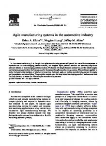
transferred). This relationship Pallet transfer is one-to-one from transfer site to Pallet desc. The relationship Pallet transfer has four main attributes, Pallet id, Site id, Activity, Pallet trans time. Pallet transfer is uniquely identi ed by Pallet id and Site id. Figure 4 shows the entity-relationship diagram of the agile database system.
4.2 Conversion from the E-R Model to the Relational Data Model We now convert the entity-relationship diagram of Figure 4 to a relational database scheme. The following are the relation schemes for the entity set. Each relation comes from the entity set with the same name. Assembled part(Assem part id, Assem part name, Worktables, Gripper type) Robot(Rob id,Rob spec) Raw part(Raw part id, Raw part name, Height, Diameter)
Chapter 1
18
Assem_action
Rob_id Assem_part_id
S_assem_time
F_assem_time
Curly
A000000001
Put_Handle
12:25:13
12:25:15
Curly
A000000002
Put_Tran_Hold
12:25:19
12:25:23
Curly
B000000001
Put_Ter_Screw
12:25:28
12:25:30
Larry
C000000001
Put_Tran_Unit
13:01:23
13:01:26
Larry
D000000001
Put_Tran_Cap
13:01:42
13:01:45
No Null Constraint (No tuple may contain a null value for this attribute)
Figure 5
No Null Integrity Constraints.
Camera(Camera id, Camera spec) Feeder(Feeder id, Feeder spec) Pallet desc(Pallet id, Pallet spec) Transfer site(Site id, Site spec) We consider the relationship in Figure 4. The relationships yield the following relation schemes. Robot assem(Rob id, Assem part id, Assem action, S assem time, F assem time) Pictures(Camera id, Raw part id, Picture time) Provides(Feeder id, Raw part id, Provide time) Robot get(Rob id, Raw part id, Get time) Robot move(Assem part id, Rob id, Pallet id, From, To, Start move time, Finish move time) Pallet transfer(Pallet id, Site id, Activity, Pallet trans time) The set of attributes forming the primary key of each relation is indicated by boldface letters.
5 INTEGRITY CONSTRAINTS We now discuss domain constraints for the actual values stored in the database. A domain constraint states that the values of a particular attribute are de ned on the set of values of a particular domain. The integrity constraints we use impose restrictions on values of attributes as follows: 1. No-null constraints : No nulls are allowed in an attribute of a relation table.
Real-Time Database In Agile Manufacturing
19
Relation Robot Rob_id
Rob_spec
Curly
Adept550
Larry
Adept550
Moe
AdeptOne Unique Key Constraint (No tuple may duplicate a value in the constraints attribute)
Figure 6
A Unique Key Constraint.
2. Unique key constraints : No two rows of a relation table have duplicate values in a speci ed attribute or a set of attributes. 3. Primary key constraints : No two rows of a relation have duplicate values in a speci ed attribute or a set of attributes, and the primary key attributes do not allow nulls (that is, a value must exist for the primary key attributes in each row). Each relation table has at most one primary key constraint. An attribute (or a set of attributes) included in the de nition of primary key integrity constraint is called the primary key. 4. Minimum (Maximum) value constraints : No value in a speci c attribute or a set of attributes is less than a minimum value (or more than a maximum value). As an example, we can de ne a no-null constraint which requires that a value be input in the Rob id attribute for every tuple of the Robot assem relation. Figure 5 illustrates a no-null integrity constraint. As an example for the unique-key constraint, consider the Robot table of Figure 6. A Unique key constraint is de ned on the Robot id attribute to disallow tuples with duplicate Robot identi cations. Figure 7 illustrates Primary Key Constraints for the Robot relation, and gives two tuples that can not be inserted into the robot relation.
6 DATA LOGGING TECHNIQUES There are two kinds of data in our environment; the static and the operational data. The operational data is generated while running the agile manufacturing system.
Chapter 1
20
Primary Key Constraint
Relation Robot Rob_id
Rob_spec
Curly
Adept550
Larry
Adept550
Moe
AdeptOne
Curly
AdeptTwo
This tuple is not allowed because "Curly" duplicates an existing value in the primary key .
Adept550
This tuple is not allowed because it contains a null value for the primary key.
Figure 7
A Primary Key Constraint.
Assem_part_id
Asseem_part_name
A000000001
Subass1
Gripper_type Handle_Gripper
A000000002
Subass1
Tran_Hold_Gripper
B000000001
Subass2
Ter_Screw_Gripper
C000000001
Subass3
Trans_Unit_Gripper
D000000001
Subass4
Trans_Cap_Gripper
Subass1=Handle + Tran_Hold
Subass2=Subass1 + Ter_Screw
Subass3=Subass2 + Tran_Unit
Subass4=Subass3 + Tran_Cap
Figure 8
The Static Data of Assembled part().
6.1 Static Data The agile database system keeps the static data in the relational database scheme, namely Assembled part(), Robot(), Raw part(), Supplier(), Pallet Desc() and Transfer site(). The static data of Assembled part() is shown in Figure 8.
6.2 Operational Data The agile system records the operational data of Robot assem such as Robotidenti cation, Assembled-part-identi cation, Assembled-part-name, Assembledaction, Worktables, Start-assembled-time and Finish-assembled-time. Figure 9 shows the operational data of Robot assem. In Figure 9, Robot "curly" assembles "Handle" on worktable 1 starting from 12:25:28 to 12:25:30.
Real-Time Database In Agile Manufacturing
21
S_assem_time
F_assem_time
Curly
A000000001
Put_Handle
12:25:13
12:25:15
Curly
A000000002
Put_Tran_Hold
12:25:19
12:25:23
Curly
B000000001
Put_Ter_Screw
12:25:28
12:25:30
Larry
C000000001
Put_Tran_Unit
13:01:23
13:01:26
Larry
D000000001
Put_Tran_Cap
13:01:42
13:01:45
Rob_id Assem_part_id
Figure 9
Assem_action
The Operational Data of Robot assem().
Example 6.1 : Let us show how the data is recorded in a relational database scheme when a robot works:
1. Grab : The data is recorded in relation Robot get(curly, A000000001, Handle, 12:25:05). Robot (curly) picks the part (Handle) at 12:25:05. 2. Move : The data is recorded in relation Robot move(A000000001, Curly, Pallet3, Subass1, Pallet3, table1, 12:25:12,12:25:16). Robot (curly) moves the part (handle) on pallet 3 to workstation 1 stating from 12:25:12 to 12:25:16. 3. Assemble : The data is recorded in relation Robot assem(Curly, A000000001, Subass1, Put Handle, table1, 12:25:13, 12:25:15). Robot (curly) does assemble handle starting from 12:25:13 to 12:25:15. 4. Move : The data is recorded in relation Robot move(A00000001, Curly, Pallet3, Subass1, Table1, Pallet3, 12:25:45, 12:25:49). Robot (Curly) moves the subassembly (handle) on workstation 1 to pallet 3 from 12:25:45 to 12:25:49. Two methods are provided to send this data to the agile database server over a network: 1 the o�-line method: The data is stored into a speci c le which is then sent to the agile database server. 2 the on-line method: A TCP/IP reply packet is created on-line which contains all the data and is sent over the network to the agile database server.
Chapter 1
22
7 EXAMPLES 7.1 Example Queries In CASE-DB, each RA query has the keyword parameter \Time=" which speci es the time constraint (or time quota), and the keyword parameter \Risk" which speci es the risk of overspending. Below we give three real-time query examples from our domain. Example 7.1 : List in 5 seconds the number of subassemblies generated by robot1 in the last 10 hours, with the risk at 0.5. Example 7.2 : List in 2 seconds the number of parts robot2 has consumed in the last 30 minutes, with the risk at 0.5. Example 7.3 : List in 2 seconds the types of worktables robot2 has used in the last 2 hours, with the risk at 0.5.
7.2 Processing Real-time Queries in Distributed-CASE-DB We de ne a real-time query as a query that needs to be evaluated within a given time deadline. A real-time query is modi ed by replacing the relations with their subrelations. The user or the database administor identi es relations that whould probably be used in real-time query processing, and divides each relation into subrelations. Figure 10 illustrates subrelations of R and S. In Figure 10, f1 � f2 � f3 � f4 and fi = fi ? fi?1 where i = 2, 3, 4. Below we illustrate with an example the way in which real-time queries are processed. We rst give a de nition. 0
De nition: Let f and g be two subrelations. Then the disjoint union ] of f and g is de ned as f ] g � f [ g where f \ g = ; In the 1st iteration, the query is evaluated with the subrelation f1 and g1 (required subrelaton) and the given amount of time. In the 2nd iteration, CASEDB computes sel2+ (the selectivity [20] used in the time cost formula) using the given risk and the selectivity obtained in the previous iteration. CASE-DB estimates the time cost of the query with di�erent subrelations and choose the subrelation(s) where the estimated time cost comes closest to and is less than the available time. Finally, CASE-DB evaluates the query with the selected subrelation(s). If the time quota is overspent before the completion of the 2nd iteration, the response obtained in the 1st iteration is returned to the user. If
Real-Time Database In Agile Manufacturing
f4
g4
f3
g3
f2
g2
f1
g1
Figure 10
23
Subrelations of R and S.
the 2nd iteration completes and the time quota runs out, the response obtained in the 2nd iteration is returned, and so on.
Example 7.4 : Consider a single join [20] operation (1) query Q with subrelation chains for relations R and S on three server sites. Consider the query Q = \List all attributes of (R 1 S) in 10 seconds with the risk at 0.5 or less" which is speci ed in RA as Q = (R 1 S ) Risk = 0:5 Time = 10sec Initially, there is no data transfer because data is stored at each server site. Each subrelation is partitioned a priori into disjoint fragments on partition attribute(s). In the rst step, query Q1 =(f1 1 g1) (which uses the smallest possible subrelations of R and S), a revised version of Q, is evaluated in parallel simultaneously without data transfer on three server sites as follows. Q1 = (f1 1 g1 )
Step 1-a (Subrelation Selection) : Site 1 does subrelation selection, and broadcasts others the result. The subrelation list F1 = ff1; g1 g is chosen
to evaluate f1 1 g1 , which constitutes the rst iterative evaluation step (with no risk analysis). Step 1-b (Partition Strategy) : Each of f1 and g1 is partitioned (a priori) into 3 disjoint fragments on the partition attribute(s) of f1 and g1 , and we have f1 = f11 ] f12 ] f13 and g1 = g11 ] g12 ] g13 . Case 1: The partition attribute(s) is the same as the join attribute(s) of f1 and g1 . f1 1 g1 = ; when i 6= j: For join processing, site 1 decides that, say, (i) Site 1 will choose the fragments f11 and g11 , (ii) Site 2 will choose the fragments f12 and g12 and (iii) Site 3 will choose the fragments f13 and g13 . i
j
Chapter 1
24
Case 2: The partition attribute(s) is di�erent from the join attribute(s) of f1 and g1 . For join processing, site 1 decides that, say, (i) Site 1 will choose the fragments f11 and g1 , (ii) Site 2 will choose the fragments f12 and g1 and (iii) Site 3 will choose the fragments f13 and g1 .
Step 1-c (Local Operation Phase) : Case 1: The partition attribute(s) is the same as the join attribute(s) of
f1 and g1 : Thus (i) Site 1 will evaluate I1 = (f11 1 g11 ), (ii) Site 2 will evaluate I2 = (f12 1 g12 ) and (iii) Site 3 will evaluate I3 = (f13 1 g13 ).
Case 2: The partition attribute(s) is di�erent from the join attribute(s)
of f1 and g1 . Then (i) Site 1 will evaluate I1 = (f11 1 g1), (ii) Site 2 will evaluate I2 = (f12 1 g1 ) and (iii) Site 3 will evaluate I3 = (f13 1 g1 ).
Step 1-d (Output Phase) : Sites 2 and 3 send their results to Site 1, and the answer to Q1 is assembled as I1 ] I2 ] I3 . This completes the rst iterative query evaluation step.
In the second iterative step, CASE-DB computes the risks of evaluating the query within the time quota with di�erent combinations of subrelations from the two subrelation chains and chooses a subrelation list with a risk that is the closest but less than the user-speci ed risk (which, in this example, is 0.5). Step 2-a (Subrelation Selection) : Site 1 does subrelation selection, and broadcasts others the result that the subrelation list F2 = ff3 ; g4 g is chosen to evaluate f3 1 g4 . Step 2-b (Partition Strategy) : f3 and g4 are each partitioned a priori into 3 disjoint fragments on the partition attribute(s) such that f1 � f3 and g1 � g4 for k = 1,2,3, and we have f3 = f31 ] f32 ] f33 and g4 = g41 ] g42 ] g43 . k
k
k
k
Case 1: The partition attribute(s) is the same as the join attribute(s) of 6 j: f3 and g4 . f3 1 g4 = ; when i = i
j
Site 1 decides that, say, Site 1 will choose the fragments f31 and g41 where f31 � f11 and g41 � g11 , Site 2 will choose the fragments f32 and g42 where f32 � f12 and g42 � g12 and Site 3 will choose the fragments f33 and g43 where f33 � f13 and g43 � g13 .
Real-Time Database In Agile Manufacturing
25
Case 2: The partition attribute(s) is di�erent from the join attribute(s)
of f3 and g4 . Site 1 decides that, say, Site 1 will choose the fragments f31 and g4 where f31 � f11 and g4 � g1 , Site 2 will choose the fragments f32 and g4 where f32 � f12 and g4 � g1 and Site 3 will choose the fragments f33 and g4 where f33 � f13 and g4 � g1 .
Step 2-c (Local Operation Phase) : Case 1: The partition attribute(s) is the same as the join attribute(s) of 6 j: f3 and g4 . f3 1 g4 = ; when i = i
j
Site 1 will evaluate J1 = (f31 1 g41 ). And, the evaluation of J1 will utilize the previous result Q1 (f11 ; g11 ) as follows: J1 = Q1 (f11 ; g11 ) ] (f11 1 (g41 ? g11 )) ] ((f31 ? f11 ) 1 g11 ) ] ((f31 ? f11 ) 1 (g41 ? g11 )) Similarly, Site 2 will evaluate J2 = (f32 1 g42 ) by rewriting J2 and utilizing Q1 (f12 ; g12 ). And, again, Site 3 will evaluate J3 = (f33 1 g43 ) by rewriting J3 and utilizing Q1 (f13 ; g13 ). Case 2: The partition attribute(s) is di�erent from the join attribute(s) of f3 and g4 . Site 1 will evaluate J1 = (f31 1 g4 ). And, the evaluation of J1 will utilize the previous result Q1 (f11 ; g1) as follows. J1 = Q1 (f11 ; g1 ) ] (f11 1 (g4 ? g1 )) ] ((f31 ? f11 ) 1 g1 ) ] ((f31 ? f11 ) 1 (g4 ? g1 )) Similarly, Site 2 will evaluate J2 = (f32 1 g4 ) and Site 3 will evaluate J3 = (f33 1 g4 ).
Step 2-d (Output Phase) : Sites 2 and 3 send their results to Site 1, and the answer to Q2 is assembled as J1 ] J2 ] J3 . There are three points to observe in example 7.4. (1) A priori fragmentation is useful when the partition attribute(s) is the same as the join attribute(s) and may not be useful otherwise. (2) There is no data transfer since each server site keeps subrelation chains for relations R and S. (3) If Q2 evaluation underspends the time quota, for the next iterations, we take very high risks so that the number of iterative query evaluation steps is reduced leading to a control on the overhead due to additional query steps.
Chapter 1
26
7.3 Rule Examples for the Coop-CASE-DB For the cooperative transaction model, two types of events are of interest: completion (of possibly intermediate steps) of a manufacturing (assembly) job and occurrences of manufacturing operation errors. The telephone socket has two pairs of wires: one short pair connects to the transmitter holder, and one long pair goes through the handle to connect the receiver unit. At the end of each wire, there is a metal pad. And the transmitter holder has two terminal screws such that the wires can be attached to the transmitter holder by touching the pad of the wire to the column of the terminal screw and tightening the terminal screw. The following are some rule examples for receiver assembly.
Rule 1: Robot1 on station 1 cooperates with Robot2 on station 2 to attach the wire pad of the socket to the terminal screw column of the transmitter holder. Robot1 holds the wire and moves the pad to touch the terminal screw column. Then, Robot2 uses a screw driver to tighten the terminal screw such that the wire pad is rmly attached to the transmitter holder. Robot1 may detect that the wire is bent and it has di�culty to hold and move the wire to the correct position at the terminal screw column. On this event (detection of a bent wire), Robot1 sends information to Robot2 so that Robot2 can utilize the time to work on other jobs. Let the event of detecting a bent wire be BentWire. Robot1 sends an estimated time RecoveryTime to recover from the problem to Robot2 . Robot2 receives the time as FreeTime and schedules other jobs for itself for the free time. The two tasks (receiving and scheduling) for Robot2 are sequential. The action has to be executed in time interval [now, now + 1 second] relevant to the event occurrence time now. The rule is speci ed as:
r1 : BentWire ! Robot1 : SEND(Robot2 , RecoveryTime); sequence [
Robot2 : RECEIVE(Robot1, FreeTime); Robot2 : ScheduleJob(FreeTime) ]
in [0, 1].
Rule 2:
Real-Time Database In Agile Manufacturing
27
A robot gets raw parts from a feeder. At the end of the feeder, there is a CCD camera to take pictures of raw parts. The pictures are processed by the vision system to provide orientation of the raw parts to the robot. An error message, NoOrientationDataError, is issued if the robot has waited for more than twenty seconds for orientation data. The error can be caused by several possible components. Below are some possible errors. There are no raw parts in the feeder. The feeder has stopped: Pictures of raw parts are not taken. The vision system is malfunctional. The vision system is overloaded: too many pictures are sent to the vision system for image processing, and the image processing task for the robot has too low a priority. On the occurrence of this event, the agile manufacturing system rst tries to locate the causes of the problem. If it can automatically recover from the problem, the system recovers by itself and reports an error for the record. Otherwise, it sends an alarm to an operator, and describes to the operator the possible causes of the problem (if it can locate the causes of the problem) as well as possible remedies to be taken by the operator. If the feeder stops, information on the feeder and raw parts from the database can be helpful to diagnose the problem. Some possible queries include 1. 2. 3. 4.
Obtain the accumulative usage of the feeder; List the maintenance record of the feeder; Print the recent diagnosis of the problem; Produce quality control report on the raw parts.
Such queries are requested while calling for an operator. A real-time time constraint (e.g., 2 seconds) is associated with each activity.
r2 : NoOrientationDataError in [-20, 0] ! sequence [
Chapter 1
28
LocateCause; SolveProblem ] in [0, 2] secs. The action SolveProblem recovers from the manufacturing error, or sends an alarm to an operator if the manufacturing error can not be recovered.
Rule 3: For summary analysis, daily and weekly reports with their respective charts on the manufacturing operation are produced at di�erent levels of detail. Weekly reports which cover the manufacturing operation of the previous ve days are produced on Mondays. Daily reports are not produced on Mondays. Sometimes, a weekly report is required on a day other than Monday for a presentation or for a review due to a manufacturing problem. No daily reports are needed when there is a weekly report. We use a rule to skip the production of a daily report.
r3 : ProduceWeeklyReport ! :ProduceDailyReport: ProduceWeeklyReport and ProduceDailyReport are queries to produce weekly reports and daily reports, respectively.
Rule 4: A socket and a transmitter unit are assembled into a subassembly Subass1. The time for this assembly varies. When it takes longer to nish the assembly, the handle supplier should not ship a handle to the station where a handle and a Subass1 are assembled. A rule specifying this requirement has a negative event \:FinishSubass1 in [-3, 0] secs", and a prohibited action \:SupplyHandle in [0, 5] secs." If the event FinishSubass1 is not received within the last three seconds, the shipment of a handle should be prohibited for the next ve seconds.
r4 : :FinishSubass1 in [-3, 0] secs ! :SupplyHandle in [0, 5] secs.
7.4 Visual Queries We now present VISUAL versions of the three queries listed in section 7.1.
Real-Time Database In Agile Manufacturing
Figure 11
29
Visual Version of Example 7.1.
Figure 11 presents the VISUAL version of the query \List in 5 seconds the number of subassemblies generated by robot1 in the last 10 hours, with the risk at 0.5". Query ASSEMBLED PARTS returns in 5 seconds with risk at 0.5, a set of assembled parts which were generated by robot1 in the last 10 hours. The Query head indicates the query name (ASSEMBLED PARTS) and the return type (Set of assembled parts). The query body contains a robot relation object with variable R and an assembled part relation object with variable AP. The fact that assembled part AP is generated by robotR is indicated by the Robot assem relation. F indicates the nish time of assembly ( nish time is before the current time); and S indicates the start time of the assembly (started at most 10 hours ago). Robot id (1), risk (0.5), and time limit (5 sec.) are indicated in three seperate condition boxes. Figure 12 presents the VISUAL version of the query \List in 2 seconds the number of parts robot2 has consumed in the last 30 minutes, with the risk at 0.5". Query NUMBER OF PARTS CONSUMED uses a sub-query (external query PARTS CONSUMED) to come up with the count of parts consumed by robot2 in the last 30 minutes. The time limit is 2 seconds and the risk is 0.5. The result of the query is an integer (X). The result X is calculated by using an aggregate function in the condition box (COUNT). The result of the external
Chapter 1
30
Figure 12
Visual Version of Example 7.2.
query PARTS CONSUMED is counted. Query PARTS CONSUMED returns a set of raw parts (RP). In the query body, a robot relation object (R) and a raw part relation object (RP) are shown. The connection between them is established by using the Robot get relation. F and S represent the start and nish times, respectively. Again the condition boxes are used to select robots with id 2 and to set the time (2 sec.) and risk (0.5) factors. Figure 13 presents the VISUAL version of the query \List in 2 seconds the types of worktables robot2 has used in the last 2 hours, with the risk at 0.5". Query WORKTABLES returns a set of worktable relation objects which are used by robot2 in the last 2 hours (in 2 seconds and with risk 0.5). A robot (R) is associated with an assembled part (AP) using the relation Robot assem. The start (S) and nish (F) times of the assembly is set to be the last 2 hours. Robot id, time limit, and risk conditions are set in condition boxes. Finally, the worktable that assembled part AP resided on is associated to output of the query (W).
Real-Time Database In Agile Manufacturing
Figure 13
31
Visual Version of Example 7.3.
8 CONCLUSIONS AND FUTURE WORK We have described an agile munufacturing system and an agile manufacturing database system designed for capturing and manipulating the operational data of a munufacturing cell. The AMDS that uses the cooperative transaction model in order for transactions to cooperative provides o�-line analysis, realtime monitoring and active interaction capabilities. We have also shown how the static and the operational data are logged and real-time (as well as nonreal-time) queries are speci ed through graphical language. Our future work includes a full implementation and empirical evaluation, which is currently being carried out.
REFERENCES [1] Adept Technology Inc., \Adept MV Controller User's Guide for Models MV-8 and MV-19", October 1994.
32
Chapter 1
[2] Adept Technology Inc., \V+ Operating System User's Guide", Version 11.0, June 1993. [3] N.H. Balkir, \Visual-A Graphical Icon-Based Query Language", M.S. thesis, CWRU, May 1995. [4] N.H. Balkir, E. Sukan, G. Ozsoyoglu, Z.M. Ozsoyoglu, \VISUAL-A Graphical Icon-Based Query Languages", 12th IEEE ICDE Conf., February 1996. [5] T.E. Bell, \The Flexible Factory: Case Studies", IEEE Spetrum, September 1993, pp. 28-42. [6] S. Chakravarthy (ed.), Special Issue on Active Databases, Bulletin of the TC on Data Engineering, Vol. 15, No. 1-4, December 1992. [7] D. Dayal, B. Blaustein, A. Buchnamm, U. Charkravarthy, M. Hsu, R. Ladin, D. McCarthy, A. Rosenthal, S. Sarin, M.J. Livny, R. Jauhari, \HiPAC Project: Combining Active Databases and Timing Constraints", SIGMOD Record, Vol. 17, No. 1, March 1988, pp. 51 - 70. [8] A. Elmagarmid (ed.), Advanced Transaction Models for New Applications, Morgan-Kaufmann, 1992. [9] N.H. Gehani, H.V. Jagadish, and O. Shmueli, \Event Speci cation in an Active Object-Oriented Database", SIGMOD Conf., 1992, pp. 81-90. [10] W-C. Hou and G. Ozsoyoglu, \Processing Real-Time Aggregate Relational Queries in CASE-DB", ACM Transaction on Database Systems, June 1993, pp. 224-261. [11] H.-C. Kuo and G. Ozsoyoglu, \Cooperative Transaction for Real-Time Databases", The Fourth International Workshop on Parallel and Distributed Real-time Systems", Honolulu, Hawaii, April 1996, pp. 110-117. [12] H.-C. Kuo and G. Ozsoyoglu, \Processing Repeating Events in Real-Time Active Databases", Technical Report, Case Western Reserve University, 1996. [13] S. Lee and G. Ozsoyoglu, \Distributed Processing of Time-Constrained Queries in CASE-DB", The Fifth International Conference on Information and Knowledge Management, November 1996. [14] K.J. Lin, \Consistency Issues in Real-Time Database Systems", 22nd Hawaii International Conference System Sciences, Hawaii, January 1989. [15] P. O'neil, \Database Principles Programming Performance", Morgan Kaufmann Publishers, Inc., 1994
Real-Time Database In Agile Manufacturing
33
[16] G. Ozsoyoglu, S. Guruswamy, K. Du, and W-C. Hou, "Time-Constrained Query Processing in CASE-DB", IEEE Transactions for Knowledge and Data Engineering, 1995. [17] R.D. Quinn, G.C. Causey, F.L. Merat, D.M. Sargent, N.A. Barendt, W.S. Newman, V.B. Velasco, A. Podgurski, J. Jo, L.S. Sterling, Y. Kim, \Design of an Agile Manufacturing Workcell for Light Mechanical Applications", Proceeding of the 1996 IEEE Internatinal Conference on Robotics and Automation, Minneapolis, MN, April 1996, pp. 858-863. [18] W.R. Stevens, \Unix Networks Programming", Prentice Hall Software Series, 1990. [19] R. Stroble and A. Johnson, \The Flexible Factory: Case Studies", IEEE Spetrum, September 1993, pp. 28-42. [20] J.D. Ullman, \Principles of Database and Knowledge-Base Systems", Vol. 1, Computer Science Press, 1988. [21] Wind River Systems Incs., \VxWorks Programmer's Guide, Version 5.3, December 1995.