Dec 23, 2014 - tion, data mining. ... time series or large datasets, dimension reduction is ...... http://nsl.unt.edu/santi/Dataset%20Collection/Data%20descr.
168
JOURNAL OF ADVANCES IN INFORMATION TECHNOLOGY, VOL. 1, NO. 4, NOVEMBER 2010
A Recent-Pattern Biased Dimension-Reduction Framework for Time Series Data Santi Phithakkitnukoon and Carlo Ratti SENSEable City Laboratory, Massachusetts Institute of Technology, Cambridge, Massachusetts, USA Email: {santi, ratti}@mit.edu
Abstract— High-dimensional time series data need dimension-reduction strategies to improve the efficiency of computation and indexing. In this paper, we present a dimension-reduction framework for time series. Generally, recent data are much more interesting and significant for predicting future data than old ones. Our basic idea is to reduce to data dimensionality by keeping more detail on recent-pattern data and less detail on older data. We distinguish our work from other recent-biased dimensionreduction techniques by emphasizing on recent-pattern data and not just recent data. We experimentally evaluate our approach with synthetic data as well as real data. Experimental results show that our approach is accurate and effective as it outperforms other well-known techniques. Index Terms— Time series analysis, dimensionality reduction, data mining.
I. I NTRODUCTION Time series is a sequence of time-stamped data points, which account for a large proportion of the data stored in today’s scientific and financial databases. Examples of a time series include stock price, exchange rate, temperature, humidity, power consumption, and event logs. Time series are typically large and of high dimensionality. To improve the efficiency of computation and indexing, dimension-reduction techniques are needed for high-dimensional data. Among the most widely used techniques are PCA (also known as SVD), DFT, and DWT. Other recently proposed techniques are Landmarks [29], PAA [21], APCS [20], PIP [15], Major minima and maxima [13], and Magnitude and shape approximation [27]. These techniques were developed to reduce the dimensionality of the time series by considering every part of a time series equally. In many applications such as the stock market, however, recent data are much more interesting and significant than old data, “recentbiased analysis” (the term originally coined by Zhao and Zhang [35]) thus emerges. The recently proposed techniques include Tilt time frame [8], Logarithmic tiltedtime window [16], Pyramidal time frame [2], SWAT [5], Equi-segmented scheme [35], and Vari-segmented scheme [35]. Generally, a time series reflects the behavior of the data points (monitored event), which tends to repeat periodically and creates a pattern that alters over time due to countless factors. Hence the data that contains the recent pattern are more significant than just recent
© 2010 ACADEMY PUBLISHER doi:10.4304/jait.1.4.168-180
data and even more significant than older data. This change of behavioral pattern provides the key to our proposed framework in dimension reduction. Since the pattern changes over time, the most recent pattern is more significant than older ones. In this paper, we introduce a new recent-pattern biased dimension-reduction framework that gives more significance to the recent-pattern data (not just recent data) by keeping it with finer resolution, while older data is kept at coarser resolution. With our framework, the traditional dimension-reduction techniques such as SVD, DFT, DWT, Landmarks, PAA, APCS, PIP, Major minima and maxima, and Magnitude and shape approximation can be used. As many applications [1] [7] [10] [24] generate data streams (e.g., IP traffic streams, click streams, financial transactions, text streams at application level, sensor streams), we also show that it is simple to handle a dynamic data stream with our framework. We distinguish this paper from other previously proposed recent-biased dimension-reduction techniques by the following contributions: 1) We develope a new framework for dimension reduction by keeping more detail on data that contains the most recent pattern and less detail on older data. 2) Within this framework, we also propose Hellinger distance-based algorithms for recent periodicity detection and recent-pattern interval detection. II. BACKGROUND AND R ELATED W ORK This section reviews traditional dimension reduction methods and briefly describes related work in the recentbiased dimension reduction. A. Dimension Reduction With advances in data collection and storage capabilities, the amount of the data that needs to be processed is increasing rapidly. To improve the efficiency of computation and indexing when dealing with high-dimensional time series or large datasets, dimension reduction is needed. The classical methods include PCA, DFT, and DWT: PCA (Principal Component Analysis) [14] is a popular linear dimension-reduction technique that minimizes the mean square error of approximating the data. It is also known as the singular value decomposition (SVD), the Karhunen-Loeve transform, the Hotelling transform, and the empirical orthogonal function (EOF) method. PCA
JOURNAL OF ADVANCES IN INFORMATION TECHNOLOGY, VOL. 1, NO. 4, NOVEMBER 2010
is an eigenvector-based multivariate analysis that seeks to reduce dimension of the data by transforming the original data to a few orthogonal linear combinations (the PCs) with the largest variance. DFT (Discrete Fourier Transform) has been used for the dimensionality reduction [3] [31] [22] [9] by transforming the original time series (of length N ) without changing information content to the frequency domain representation and retaining a few low-frequency coefficients (p, where p < N ) to reconstruct the series. Fast Fourier transform (FFT) is a popular algorithm to compute DFT with time complexity of O(N log N ). DWT (Discrete Wavelet Transform) is similar to DFT except that it transforms the time series into time/frequency domain and its basis function is not a sinusoid but generated by the mother wavelet. Haar wavelet [6] is one of the most widely used class of wavelets with time complexity of O(N ). Other proposed techniques include Landmarks, PAA, APCS, PIP, Major minima and maxima, and Magnitude and shape approximation: Landmark model has been proposed by Perng et al. [29] to reduce dimensionality of time series. The idea is to reduce the time series to the points (time, events) of greatest importance, namely ”landmarks”. The n-th order landmark of a curve is defined for the point whose n-th order derivative is zero. Hence local maxima and minima are first-order landmarks, and inflection points are second-order landmarks. Compared with DFT and DWT, landmark model retains all peaks and bottoms that normally filtered out by both DFT and DWT. Keogh et al. [21] have proposed PAA (Piecewise Aggregate Approximation) as a dimension-reduction technique that reduces the time series to the mean values of the segmented equi-length sections. PAA has an advantage over DWT as it is independent of the length of the time series (DWT is only defined for sequences whose length is an integral power of two). The concept of PAA has later been modified to improve the quality of approximation by Keogh et al. [20] who propose APCS (Adaptive Piecewise Constant Approximation) that allows segments to have arbitrary lengths. Hence two numbers are recorded for each segment; mean value and length. PIP (Perpetually Important Points) has been introduced by Fu et al. [15] to reduce dimensionality of the time series by replacing the time series with PIPs, which are defined as highly fluctuated points. Fink et al. [13] have proposed a technique for fast compression and indexing of time series by keeping major minima and maxima and discarding other data points. The indexing is based on the notion of major inclines. Ogras and Ferhatosmanoglu [27] have introduced a dimension-reduction technique that partitions the high dimensional vector space into orthogonal subspaces by taking into account both magnitude and shape information of the original vectors. © 2010 ACADEMY PUBLISHER
169
B. Recent-biased Dimension Reduction Besides the global dimension reduction, in many applications such as stock prices, recent data are much more interesting and significant than old data. Thus, the dimension-reduction techniques that emphasize more on the recent data by keeping recent data with fine resolution and old data with coarse resolution have been proposed such as Tilt time frame, Logarithmic tilted-time window, Pyramidal time frame, SWAT, Equi-segmented scheme, and Vari-segmented scheme: Tilt time frame has been introduced by Chen et al. [8] to minimize the amount of data to be kept in the memory or stored on the disks. In the tilt time frame, time is registered at different levels of granularity. The most recent time is registered at the finest granularity, while the more distant time is registered at coarser granularity. The level of coarseness depends on the application requirements. Similar to the tilt time frame concept but with more space-efficient, Giannella et al. have proposed the logarithmic tilted-time window model [16] that partitions the time series into growing tilted-time window frames at an exponential rate of two e.g., 2, 4, 8, 16, and so forth. The concept of the pyramidal time frame has been introduced by Aggarwal et al. in [2]. With this technique, data are stored at different levels of granularity depending upon the recency, which follows a pyramidal pattern. SWAT (Stream Summarization using Wavelet-based Approximation Tree) [5] has been proposed by Bulut and Singh to process queries over data streams that are biased towards the more recent values. SWAT is a Haar waveletbased scheme that keeps only a single coefficient at each level. Zhao and Zhang have proposed the equi-segmented scheme and the vari-segmented scheme in [35]. The idea of the equi-segmented scheme is to divide the time series into equi-length segments and apply a dimension reduction technique to each segment, and keep more coefficients for recent data while fewer coefficients are kept for old data. Number � of �coefficients to be kept for each segment is set to N/2i where N is the length of the time series and segment gets older with the increase of i. For the vari-segmented scheme, the time series is divided into variable length segments with larger segments for older data and smaller segments for more recent data (the length of segment i is set to 2i ). The same number of coefficients are then kept for all segments after applying a dimension reduction technique to each segment. III. R ECENT-PATTERN B IASED D IMENSION -R EDUCTION F RAMEWORK Time series data analysis comprises methods that attempt either to understand the context of the data points or to make forecasts based on observations (data points). In many applications, recent data receive more attention than old ones. Generally, a time series reflects the behavior of the data points (monitored event), which tends to repeat periodically and creates a pattern that alters over time due to countless factors. Hence the data that contains recent
170
JOURNAL OF ADVANCES IN INFORMATION TECHNOLOGY, VOL. 1, NO. 4, NOVEMBER 2010
pattern are more significant than just recent data and even more significant than older data. Typically, future behavior is more relevant to the recent behavior than older ones. Our main goal in this work is to reduce dimensionality of a time series with the basic idea of keeping data that contains recent pattern with high precision and older data with low precision. Since the change in behavior over time creates changes in the pattern and the periodicity rate, we thus need to detect the most recent periodicity rate, which will lead to identifying the most recent pattern. Hence a dimension reduction technique can then be applied. This section presents our novel framework for dimension reduction for time series data, which includes new algorithms for recent periodicity detection, recentpattern interval detection, and dimension reduction. A. Recent Periodicity Detection Unlike other periodicity detection techniques ( [4], [11], [12], [19], [23], and [33]) that attempt to detect the global periodicity rates, our focus here is to find the “most recent” periodicity rate of time series data. Let X denote a time series with N time-stamped data points, and xi be the value of the data at time-stamp i. The time series X can be represented as X = x0 , x1 , x2 , ..., xN , where x0 is the value of the most recent data point and xN is the value of the oldest data point. Let Φ(k) denote the recent-pattern periodicity likelihood (given by (1)) that measures the likelihood of selected recent time segment (k) being the recent period of the time series, given that the time series X can be sliced into equal-length k , each of length k, segments X0k , X1k , X2k , ..., X�N/k�−1 k where Xi = xik , xik+1 , xik+2 , ..., xik+k−1 . ��N/k�−1 ˆ 0k , X ˆ k )) (1 − d2H (X i , (1) Φ(k) = i=1 �N/k� − 1 where d2H (A, B) is Hellinger distance [32], which is widely used for estimating a distance (difference) between two probability measures (e.g., probability density functions (pdf), probability mass functions (pmf)). Hellinger distance between two probability measures A and B can be computed by (2). A and B are M -tuple {a1 , a2 , a3 , ..., aM } � and {b1 , b2 , b3 , ..., bM } respectively, � and satisfy am ≥ 0, m am = 1, bm ≥ 0, and m bm = 1. Hellinger distance of 0 implies that A = B whereas disjoint A and B yields the maximum distance of 1. M � 1 � √ d2H (A, B) = ( am − bm )2 . 2 m=1
(2)
ˆ 0k and X ˆ k are X0k and X k after norIn our case, X i i malization, respectively, such that they satisfy the above conditions. Thus, Φ(k) has the values in the range [0, 1] as 0 and 1 imply the lowest and the highest recent-pattern periodicity likelihood, respectively. Definition 1. If a time series X of length N can be sliced into equal-length p segmentsX0p , X1p , X2p , ..., X�N/p�−1 , each of length © 2010 ACADEMY PUBLISHER
p, where Xip = xip , xip+1 , xip+2 , ..., xip+p−1 , and p = arg max Φ(k), then p is said to be the recent k
periodicity rate of X. The basic idea of this algorithm is to find the time segment (k) that has the maximum Φ(k), where k = 2, 3, ..., �N/2�. If there is a tie, smaller k is chosen to favor shorter periodicity rates, which are more accurate than longer ones since they are more informative [12]. The detailed algorithm is given in Fig. 1. Note that Φ(1) = 1 ˆ 1, X ˆ 1 ) = 0, hence k begins at 2. since d2H (X 0 i p = PERIODICITY(X) Input: Time series (X) of length N Output: Recent periodicity rate (p) 1. FOR k = 2 to �N/2� 2. Compute Φ(k); 3. END FOR 4. p = k that maximizes Φ(k); 5. IF |k|> 1 6. p = min(k); 7. END IF 8. Return p as the recent periodicity rate; Figure 1. Algorithm for the recent periodicity detection.
B. Recent-Pattern Interval Detection After obtaining the recent periodicity rate p, our next step towards dimension reduction for a time series X is to detect the time interval that contains the most recent pattern. This interval is a multiple of p. We base our detection on the shape of the pattern and the amplitude of the pattern. For the detection based on the shape of the pattern, we construct three Hellinger distance-based matrices to measure the differences within the time series as follows: 1) D1i = [d1 (1), d1 (2), ..., d1 (i)] is the matrix whose elements are Hellinger distances between the patp ¯p tern derived from the X0p to Xj−1 (X 0→j−1 ), which can be simply computed as a mean time series over time segments 0 to j − 1 given by (4), and the pattern captured within the time segment j (Xjp ) as follows: ˆ¯ p ˆ p ), d1 (j) = d2 (X ,X (3) H
0→j−1
j
where j−1 j−1 j−1 1� 1� 1� p ¯ X0→j−1 = xnp , xnp+1 , ..., xnp+p−1 . j n=0 j n=0 j n=0 (4) Again, the hat on top of the variable indicates the normalized version of the variable. 2) D2i = [d2 (1), d2 (2), ..., d2 (i)] is the matrix whose elements are Hellinger distance between the most recent pattern captured in the first time segment (X0p ) and the pattern occupied within the time segment j (Xjp ) as follows:
ˆ p, X ˆ p ). d2 (j) = d2H (X 0 j
(5)
JOURNAL OF ADVANCES IN INFORMATION TECHNOLOGY, VOL. 1, NO. 4, NOVEMBER 2010
�N/p�−1
�N/p�−1
171
�N/p�−1
rshape = SHAPE RPI(D1 ,D2 ,D3 ) �N/p�−1 �N/p�−1 �N/p�−1 ,D2 , D3 ). Input: Three distance matrices (D1 Output: Shape-based recent-pattern interval (rshape ). 1. Initialize rshape to N 2. FOR i = 2 to �N/p� − 1 3. IF SIG CHANGE(D1i ,d1 (i+1)) + SIG CHANGE(D2i ,d2 (i+1)) + SIG CHANGE(D3i ,d3 (i+1)) ≥ 2 4. rshape = ip; 5. EXIT FOR LOOP 6. END IF 7. END FOR 8. Return rshape as the recent-pattern interval based on the shape; Figure 2. Algorithm for detecting the recent-pattern interval based on the shape of the pattern.
3) D3i = [d3 (1), d3 (2), ..., d3 (i)] is the matrix whose elements are Hellinger distance between the adjacent time segments as follows: ˆp , X ˆ p ). d3 (j) = d2H (X j−1 j
(6)
These three matrices provide the information on how much the behavior of the time series changes across all time segments. The matrix D1i collects the degree of difference that Xjp introduces to the recent segment(s) of the time series up to j = i, where j = 1, 2, 3, ..., �N/p�− 1. The matrix D2i records the amount of difference that the pattern occupied in the time segmentXjp makes to the most recent pattern captured in the first time segmentX0p up to j = i. The matrix D3i keeps track of the differences between the patterns captured in the adjacent time p and Xjp up to j = i. segmentsXj−1 To identify the recent-pattern interval based on the shape of the pattern, the basic idea here is to detect the first change of the pattern that occurs in the time series as we search across all the time segments Xjp in an increasing order of j starting from j = 1 to �N/p� − 1. Several changes might have been detected as we search through entire time series, however our focus is to detect the most recent pattern. Therefore, if the first change is detected, the search is over. The change of pattern can be observed from the significant changes of these three matrices. The significant change is defined as follows. Definition 2. If µDki and σDki is the mean and the standard deviation of Dki and µDi + 2σDi ≤ dk (i + 1), k k p then Xi+1 is said to make the significant change based on its shape. With the detected significant changes in these distance matrices, the recent-pattern interval based on the shape of the pattern can be defined as follows. The detailed algorithm is given in Fig. 2. p introduces a significant change to Definition 3. If Xi+1 at least two out of three matrices (D1i ,D2i , and D3i ), then the recent-pattern interval based on the shape (rshape ) is said to be ip time units.
For this shape-based recent-pattern interval detection, the Hellinger distances are computed by taking the nor© 2010 ACADEMY PUBLISHER
y = SIG CHANGE(Dki ,dk (i + 1)) Input: Distance matrix (Dki ) and the corresponding distance elementdk (i + 1). Output: Binary output (y) of 1 implies that there p and 0 implies is a significant change made by Xi+1 otherwise. 1. IF µDki + 2σDki ≤ dk (i + 1) 2. y = 1; 3. ELSE 4. y = 0; 5. END IF Figure 3. Algorithm for detecting the significant change.
malized version of the patterns in the time segments. Since normalization rescales the amplitude of the patterns, the patterns with similar shapes but significantly different amplitudes will not be detected (see an example illustrated in Fig. 4).
Figure 4. An example of misdetection for the recent-pattern interval based on the shape of the pattern. SHAPE RPI(algorithm given in Fig. 3) would detect the change of the pattern at the 5th time segment (X5p ) whereas the actual significant change takes place at the 3rd time segment (X3p ).
To handle this shortcoming, we propose an algorithm to detect the recent-pattern interval based on the amplitude of the pattern. The basic idea is to detect the significant change in the amplitude across all time segments. To achieve this goal, let Ai = [a(1), a(2), ..., a(i)] denote a matrix whose elements are mean amplitudes of the patterns of each time segment up to time segment i, which
172
JOURNAL OF ADVANCES IN INFORMATION TECHNOLOGY, VOL. 1, NO. 4, NOVEMBER 2010
can be easily computed by (7). a(k) =
p−1 1� x(k−1)p+n . p n=0
(7)
Similar to the previous case of distance matrices, the significant change in this amplitude matrix can be defined as follows. Definition 4. If µAi and σAi is the mean and the standard deviation of Ai and µAi + 2σAi ≤ a(i + 1), then p Xi+1 is said to make the significant change based on its amplitude. Likewise, with the detected significant change in the amplitude matrix, the recent-pattern interval based on the amplitude of the pattern can be defined as follows. The detailed algorithm is given in Fig. 5. p Definition 5. If Xi+1 makes a significant change in the i matrix (A ), then the recent-pattern interval based on the amplitude (ramp ) is said to be ip time units.
dimension reduction technique to each time segment and then keeps more coefficients for data that carries recentbehavior pattern and fewer coefficients for older data. Let Ci represent the number of coefficients retained for the time segment Xip . Since our goal is to keep more coefficients for the recent-pattern data and fewer coefficients for older data, a sigmoid function (given by (8)) is generated and centered at R time units (where the change of behavior takes place). f (t) =
1 . 1 + α−t/p
(8)
The decay factor (α) is automatically tuned to change adaptively with the recent-pattern interval (R) by being set to α = p/R, such that a slower decay rate is applied to a longer R and vice versa. The number of coefficients for each time segment can be computed as the area under the sigmoid function over each time segment (given by (9)), so the value of Ci is within the range [1, p]. �� � f (t)dt . (9) Ci = Xip
ramp = AMP RPI(A�N/p�−1 ) Input: The amplitude matrix (A�N/p�−1 ). Output: Amplitude-based recent-pattern interval (ramp ). 1. Initialize ramp to N 2. FOR i = 2 to �N/p� − 1 3. IF SIG CHANGE(Ai ,a(i + 1)) = 1 4. ramp = ip; 5. EXIT FOR LOOP 6. END IF 7. END FOR 8. Return ramp as the recent-pattern interval based on the amplitude; Figure 5. Algorithm for detecting the recent-pattern interval based on the amplitude of the pattern.
Ci decreases according to the area under the sigmoid function across each time segment as i increases, hence C0 ≥ C1 ≥ C2 ≥ ... ≥ C�N/p�−1 . Several dimension reduction techniques can be used in our framework. Among the most widely popular techniques are DFT and DWT. For DFT, we keep the first Ci coefficients that capture the low-frequency part of the time series for each time segment (some other techniques for selecting DFT coefficients such as selecting the largest Ci coefficients to preserve the energy [26] or selecting the first largest Ci coefficients [34] can also be applied here). For DWT, the number of coefficients can be computed by
(9) and rounded to the closest integer v, where v = 2pj and j = {0, 1, 2, ..., log2 p}, i.e., v ∈ {p, p2 , 2p2 , 2p3 , ..., 1}. A larger v is chosen if there is a tie.
Finally, the recent-pattern interval can be detected by considering both shape and amplitude of the pattern. Based on the above algorithms for detecting the interval of the most recent pattern based on the shape and the amplitude of the pattern, the final recent-pattern interval can be defined as follows. Definition 6. If rshape is the recent-pattern interval based on the shape of the pattern and ramp is the recent-pattern interval based on the amplitude of the pattern, then the final recent-pattern interval(R) is the lowest value among rshape and ramp − i.e., R = min(rshape , ramp ). C. Dimension Reduction
Figure 6. Recent-pattern biased dimension-reduction scheme for time series data. A time series is partitioned into equal-length segments of length p (recent periodicity rate) and more coefficients are taken for recent-pattern data and fewer coefficients are taken for older data based on the decay rate of a sigmoid function (f (t)). For this example, recentpattern interval (R) is assumed to be (i + 1)p.
Our main goal in this work is to reduce dimensionality of a time series. The basic idea is to keep more details for recent-pattern data, while older data kept at coarser level. Based on the above idea, we propose a dimensionreduction scheme for time series data that applies a
With this scheme, a time series data can be reduced by keeping the more important portion of data (recentpattern data) with high precision and the less important data (old data) with low precision. As future behavior is generally more relevant to the recent behavior than old
© 2010 ACADEMY PUBLISHER
JOURNAL OF ADVANCES IN INFORMATION TECHNOLOGY, VOL. 1, NO. 4, NOVEMBER 2010
173
Z = DIMENSION REDUCTION(X) Input: A time series (X) of length N . Output: A reduced time series (Z). 1. p = PERIODICITY(X); 2. Partition X into equal-length segments, each of length p; �N/p�−1 �N/p�−1 �N/p�−1 3. Compute matrices D1 , D3 , and A�N/p�−1 ; , D2 �N/p�−1 �N/p�−1 �N/p�−1 4. rshape = SHAPE RPI(D1 ,D2 ,D3 ); 5. ramp = AMP RPI(A�N/p�−1 ); 6. R = min(rshape , ramp ); 7. Place a sigmoid function f (t) at R; 8. FOR each segment i 9. Coef s = apply dimension-reduction technique for segment i; 10. Compute Ci ; 11. zi = first Ci Coef s; 12. END FOR /* Series of selected coefficients */ 13. Z = {z0 , z1 , z2 , ..., z�N/p�−1 }; 14. Return Z as the reduced time series; Figure 7. Algorithm for detecting the recent-pattern interval based on the amplitude of the pattern.
ones, maintaining the old data at low detail levels might as well reduces the noise of the data, which would benefit predictive modeling. This scheme is shown in Fig. 6, and the detailed algorithm is given in Fig. 7. Note that if no significant change of pattern is found in the time series, our proposed framework will work similarly to equi-segmented scheme as our R is initially set to N (by default, see Fig. 2, Fig. 5 and Definition 6). Hence the entire series is treated as a recent-pattern data, i.e., more coefficients are kept for recent data and fewer for older data according to (the left-hand side from the center of) the sigmoid function with decay factor α = p/R. It is simple to handle dynamic data streams with our framework. When new data arrive, they are kept in a new l until there are p new data points, i.e., segment Xnew l = p. If R = sp, then only the first s + 1 segments p ˜ p, X ˜ p , ..., X ˜ p ) need to be processed while ,X (Xnew 0 1 s−1 ˜ p denotes other segments remain unchanged. Note that X i a reconstructed segment i. The new reconstructed segment ˜ p , and other segments’ ˜ p will then become a new X X new 0 ˜ p becomes X ˜ p ). If order are incremented by one (e.g., X 0 1 the original time series has N data points, then the new reconstructed time series is of length N + p. An example is given in Fig. 8. IV. P ERFORMANCE A NALYSIS This section contains the experimental results to show the accuracy and effectiveness of our proposed algorithms. In our experiments, we exploit synthetic data as well as real data. The synthetic data are used to inspect the accuracy of the proposed algorithms for detecting the recent periodicity rate and the recent-pattern interval. This experiment aims to estimate the ability of proposed algorithms in detecting p and R that are artificially embedded into the synthetic data at different levels of noise in the data (measured in terms of SNR (signal-to-noise ratio) in dB). For a © 2010 ACADEMY PUBLISHER
Figure 8. An example of processing a dynamic data stream. (1) Original data has 7p data points. (2) Suppose that R = 3p. (3) New data l points are kept in a new segment Xnew until l = p, then the first R + p data points are processed with other data points unchanged. (4) The reconstructed time series of length 8p. (5) The new reconstructed p ˜ p , and other segments’ order are ˜ new becomes a new X segment X 0 incremented by one.
synthetic time series with known p and R, our algorithms compute estimated periodicity rate (˜ p) and recent-pattern ˜ and compare with the actual p and R to see if interval (R) the estimated values are matched to the actual values. We generate 100 different synthetic time series with different values of p and R. The error rate is then computed for each SNR level (0dB to 100dB) as the number of incorrect estimates (Miss) per total number of testing data, i.e. Miss/100. The results of this experiment are shown in Fig. 9. The error rate decreases with increasing SNR as expected. Our recent periodicity detection algorithm performs with no error above 61dB while our recentpattern interval detection algorithm performs perfectly above 64dB. Therefore, based on this experiment, our proposed algorithms are effective at SNR level above 64dB. We implement our algorithms on three real time series
174
JOURNAL OF ADVANCES IN INFORMATION TECHNOLOGY, VOL. 1, NO. 4, NOVEMBER 2010
240
0.4
220
Recent−pattern interval (R) Periodicity rate (p)
0.35
200 180 160
0.3 140 120
Error rate
0.25 100 80
0.2
60
12
24
36
48
60
72
84
96
108
120
132
144
156
168
180
192
204
216
228
240
252
264
276
0.15
Figure 11. A monthly water usage during 1966-1988 with detected p = 12 and R = 2p = 24.
0.1 0.05
2
0
10
20
30
40
50 60 SNR (dB)
70
80
90
1.8
100
1.6 1.4
Figure 9. Experimental result of the error rate at different SNR levels of 100 synthetic time series (with known p and R).
1.2 1 0.8 0.6 0.4
data. The first data contains the number of phone calls (both made and received) on time-of-the-day scales on a monthly basis over a period of six months (January 7th , 2008 to July 6th , 2008) of a mobile phone user [30]. The second data contains a series of monthly water usage (ml/day) in London, Ontario, Canada from 1966 to 1988 [17]. The third data contains Quarterly S&P 500 index values taken from 1900-1996 [25]. Figure 10 shows a time series of a mobile phone usage with computed p = 24 and R = 3p = 72 based on our algorithms. Likewise, Fig. 11 shows a time series of a monthly water usage with computed p = 12 and R = 2p = 24. Similarly, Fig. 12 depicts a time series of quarterly S&P 500 index values during 1900-1996 with computed p = 14 and R = 3p = 42. Based on a visual inspection, one can clearly identify that the recent periodicity rates are 24, 12, and 14; and recent-pattern intervals are 3p, 2p, and 3p for Fig. 10, Fig. 11, and Fig. 12, respectively, which shows the effectiveness of our algorithms.
0.2
14
28
42
56
70
84
98
112 126 140 154 168 182 196 210 224 238 252 266 280 294 308 322 336 350 364 378 388
Figure 12. Quarterly S&P 500 index values taken from 1900-1996 with detected p = 14 and R = 3p = 42.
we are able to reduce much more data. In fact, there are 276 data points of water usage data before the dimension reduction and only 46 data points are retained afterward by using DFT and 52 data points kept using DWT, which is 83% and 81% reduction, respectively. Likewise, for the S&P 500 data, we are able reduce 83% of data by keeping 66 DFT coefficients and 81% by keeping 72 DWT coefficients from the original data of length 378. The reconstructed time series using DFT and DWT for mobile phone data, water usage data, and S&P 500 data are shown in Fig. 13(a) and (b), Fig. 14(a) and (b), and Fig. 15(a) and (b), respectively. 35
30 35
25
30
20
25
15
20
10
15
5
10
0
24
48
72
96
120
144
72
96
120
144
5
0
24
48
72
96
120
(a)
144 35
Figure 10. A monthly mobile phone usage over six months (January 7th , 2008 to July 6th , 2008) with detected p = 24 and R = 3p = 72.
30
25
20
We implement our recent-pattern biased dimensionreduction algorithm on these three real time series data. Due to the space limitation, the experimental results are only illustrated with DFT and DWT as the dimensionreduction techniques. As the results, the 144-point mobile phone data has been reduced to 75 data points using DFT, which is 48% reduction, and reduced to 70 points using Haar DWT, which is 51% reduction. For the water usage data, since it has a relatively short recent-pattern interval compared to the length of its entire series thus © 2010 ACADEMY PUBLISHER
15
10
5
0
24
48
(b) Figure 13. (a) The reconstructed time series of the mobile phone data of 75 selected DFT coefficients from the original data of 144 data points, which is 48% reduction. (b) The reconstructed time series of the mobile phone data with 51% reduction by keeping 70 DWT coefficients from the original data of 144 data points.
JOURNAL OF ADVANCES IN INFORMATION TECHNOLOGY, VOL. 1, NO. 4, NOVEMBER 2010
220
2
200
1.8
175
1.6 180
1.4 160
1.2 140
1 120
0.8 100
80
0.6
12
24
36
48
60
72
84
96
108
120
132
144
156
168
180
192
204
216
228
240
252
264
276
0.4
14
28
42
56
70
84
98
(a)
(a) 240
2
220
1.8
200
1.6
180
1.4
160
1.2
140
1
120
0.8
100 80
112 126 140 154 168 182 196 210 224 238 252 266 280 294 308 322 336 350 364 378
0.6
12
24
36
48
60
72
84
96
108
120
132
144
156
168
180
192
204
216
228
240
252
264
276
0.4
14
28
42
56
70
84
98
112 126 140 154 168 182 196 210 224 238 252 266 280 294 308 322 336 350 364 378
(b)
(b)
Figure 14. (a) The reconstructed time series of the water usage data of 46 selected DFT coefficients from the original data of 276 data points, which is 83% reduction. (b) The reconstructed time series of the water usage data with 81% reduction by keeping 52 DWT coefficients from the original data of 276 data points.
Figure 15. (a) The reconstructed time series of the S&P 500 data of 66 selected DFT coefficients from the original data of 378 data points, which is 83% reduction. (b) The reconstructed time series of the S&P 500 data with 81% reduction by keeping 72 DWT coefficients from the original data of 378 data points.
To compare the performance of our proposed framework with other recent-biased dimension-reduction techniques, a criterion is designed to measure the effectiveness of the algorithm after dimension reduction as following. ˜ are the original and reconDefinition 7. If X and X structed time series, respectively, then the “recent-pattern biased error rate” is defined as ˆ˜ ˜ = B · d2 (X, ˆ X) ErrRP B (X, X) H �� 2 �N/p�−1 1 � ˆ˜i , = x ˆi − x b(i) 2 i=0 (10) where B is a recent-pattern biased vector (which is a sigmoid function in our case). ˜ are the original and reconDefinition 8. If X and X ˜ is structed time series, respectively and ErrRP B (X, X) the recent-pattern biased error rate, then the Reductionto-Error Ratio (RER) is defined as RER =
P ercentage Reduction . ˜ ErrRP B (X, X)
(11)
We compare the performance of our recent-pattern biased dimension-reduction algorithm (RP-DFT/DWT) to equi-DFT/DWT, vari-DFT/DWT (with k = 8 [35]), and SWAT as we apply these algorithms on the mobile phone, water usage, and S&P 500 data. Table 1 shows the values of percentage reduction, recent-pattern biased error rate, and RER for each algorithm based on DFT. It shows that SWAT has the highest reduction rates as well as the highest error rates in all three data. For the mobile phone data, the values of the percentage reduction are the same for our RP-DFT and equi-DFT because R is exactly a half of the time series hence the sigmoid function is placed at the half point of © 2010 ACADEMY PUBLISHER
the time series (N/2) that makes it similar to equi-DFT (in which the number of coefficients is exponentially decreased). The error rate of our RP-DFT is however better than equi-DFT by keeping more coefficients particularly for the “recent-pattern data” and fewer for older data instead of keeping more coefficients for just recent data and fewer for older data. As a result, RP-DFT performs with the best RER among others. For the water usage data, even though RP-DFT has a higher error rate than equi-DFT, R is a relatively short portion with respect to the entire series thus RP-DFT is able to achieve much higher reduction rate, which results in a better RER and the best among others. For S&P 500 data, our RP-DFT is able to reduce more data than equi-DFT and vari-DFT with the lowest error rate, hence it has the highest RER. Likewise, Table 2 shows the values of percentage reduction, recent-pattern biased error rate, and RER for each algorithm based on DWT. Similar to the results of the DFT-based algorithms, our proposed RP-DWT performs with the best RER among other algorithms in all three data. One may notice that the values of the percentage reduction are different from DFT-based algorithms. This is due to the rounding process of Ci to the closest integer v (described in Section 3.3). Furthermore, we perform additional experiments on 30 more real time series , which represent data in finance, health, chemistry, hydrology, industry, labour market, macro-economic, and physics. These data are publicly available at the “Time Series Data Library [18],” which has been created by professor Rob J. Hyndman from Monash University. Our RP-DFT/DWT also show better performance than other techniques for all 30 time series data (the results are shown in the Appendix). In addition to the results of the performance compar-
176
JOURNAL OF ADVANCES IN INFORMATION TECHNOLOGY, VOL. 1, NO. 4, NOVEMBER 2010
TABLE I. P ERFORMANCE COMPARISON OF OUR PROPOSED RP-DFT AND OTHER WELL - KNOWN TECHNIQUES ( EQUI -DFT, VARI -DFT, AND SWAT) BASED ON P ERCENTAGE R EDUCTION , R ECENT- PATTERN BIASED ERROR RATE (ErrRBP ), AND RER FROM THE REAL DATA . Data RP-DFT
Percentage Reduction equi-DFT vari-DFT
SWAT
RP-DFT
ErrRBP equi-DFT vari-DFT
SWAT
RP-DFT
RER equi-DFT vari-DFT
SWAT
Mobile phone
0.479
0.479
0.750
0.972
0.0175
0.0301
0.0427
0.192
27.458
15.915
17.573
5.078
Water usage
0.837
0.479
0.739
0.986
0.00712
0.00605
0.0168
0.0641
117.550
79.201
43.996
15.375
S&P 500
0.829
0.479
0.742
0.989
0.00735
0.00739
0.00895
0.0811
112.891
64.875
82.899
12.210
TABLE II. P ERFORMANCE COMPARISON OF OUR PROPOSED RP-DWT AND OTHER WELL - KNOWN TECHNIQUES ( EQUI -DWT, VARI -DWT, AND SWAT) BASED ON
P ERCENTAGE R EDUCTION , R ECENT- PATTERN BIASED ERROR RATE (ErrRBP ), AND RER FROM THE REAL DATA .
Data RP-DWT
Percentage Reduction equi-DWT vari-DWT
SWAT
RP-DWT
ErrRBP equi-DWT vari-DWT
SWAT
RP-DWT
RER equi-DWT vari-DWT
SWAT
Mobile phone
0.514
0.500
0.750
0.972
0.0167
0.0283
0.0401
0.192
30.794
17.683
18.689
5.078
Water usage
0.812
0.493
0.739
0.986
0.00650
0.00561
0.0159
0.0650
124.852
87.854
46.565
15.152
S&P 500
0.810
0.495
0.742
0.989
0.00728
0.00711
0.00856
0.0811
111.182
69.561
87.783
12.211
ison on the real data, we generate 100 synthetic data to further evaluate our algorithm compared to the others. After applying each algorithm to these 100 different synthetic time series, Table 3 and Table 4 show the average values of percentage reduction, recent-pattern biased error rate, and RER for each algorithm based on DFT and DWT, respectively. These tables show that our proposed algorithm (both DFT-based and DWT-based) yields better RER than others. TABLE III. P ERFORMANCE COMPARISON OF OUR PROPOSED RP-DFT AND OTHER WELL - KNOWN TECHNIQUES ( EQUI -DFT, VARI -DFT, AND
SWAT) BASED ON THE AVERAGE P ERCENTAGE R EDUCTION , R ECENT- PATTERN BIASED ERROR RATE (ErrRBP ), AND RER FROM
100 SYNTHETIC DATA .
Algorithm
Percentage Reduction
ErrRBP
RER
RP-DFT equi-DFT vari-DFT SWAT
0.758 0.481 0.748 0.975
0.0209 0.0192 0.0385 0.109
36.268 25.052 19.429 8.945
V. C ONCLUSION Dimensionality reduction is an essential process of many high-dimensional data analysis. In this paper, we present a new recent-pattern biased dimension-reduction framework for time series data. With our framework, more details are kept for recent-pattern data, while older data are kept at coarser level. Unlike other recently proposed dimension reduction techniques for recent-biased time series analysis, our framework emphasizes on keeping the data that carries the most recent pattern, which is the most important data portion in the time series with a high resolution while retaining older data with a lower resolution. We show that several dimension-reduction techniques such DFT and DWT can be used with our framework. Moreover, we also show that it is simple and efficient to handle dynamic data streams with our framework. Our experiments on synthetic data as well as real data demonstrate that our proposed framework is very efficient and it outperforms other well-known recentbiased dimension reduction techniques. As our future directions, we will continue to examine various aspects of our framework to improve its performance. ACKNOWLEDGMENT
TABLE IV. P ERFORMANCE COMPARISON OF OUR PROPOSED RP-DWT AND OTHER WELL - KNOWN TECHNIQUES ( EQUI -DWT, VARI -DWT, AND
SWAT) BASED ON THE AVERAGE P ERCENTAGE R EDUCTION , R ECENT- PATTERN BIASED ERROR RATE (ErrRBP ), AND RER FROM
100 SYNTHETIC DATA .
Algorithm
Percentage Reduction
ErrRBP
RER
RP-DWT equi-DWT vari-DWT SWAT
0.745 0.488 0.748 0.975
0.0192 0.0190 0.0341 0.108
38.802 25.682 21.935 9.028
© 2010 ACADEMY PUBLISHER
The authors gratefully acknowledge support by Volkswagen of America Electronic Research Lab, the AT&T Foundation, the National Science Foundation, MIT Portugal, and all the SENSEable City Laboratory Consortium members. A PPENDIX A DDITIONAL R ESULT FOR P ERFORMANCE C OMPARISON The following are the additional results for performance comparison of our proposed method (RP-DFT/DWT) with equi-DFT/DWT, vari-DFT/DWT, and SWAT; using 30 different real time series, which represent data in finance, health, chemistry, hydrology, industry, labour market, macro-economic, and physics. These time series data
JOURNAL OF ADVANCES IN INFORMATION TECHNOLOGY, VOL. 1, NO. 4, NOVEMBER 2010
were taken from the “Time Series Data Library [18],”. Tables V and VI show the results based on DFT and DWT, respectively where Table VII gives brief description of these data. Our proposed framework shows better performance than other techniques for all 30 time series data. R EFERENCES [1] D. Abadi, D. Carney, U. Cetintemel, M. Cherniack, C. Convey, C. Erwin, E. Galvez, M. Hatoun, A. Maskey, A. Rasin, A. Singer, M. Stonebraker, N. Tatbul, Y. Xing, R. Yan, and S. Zdonik. ”Aurora: a data stream management system,” Proc. ACM SIGMOD, pp. 666, 2003. [2] C. Aggarwal, J. Han, J. Wang, and P. Yu, ”A Framework for Clustering Evolving Data Streams,” Procs. 29th Very Large Data Bases Conference (VLDB’03), pp. 81-92, Sept 2003. [3] R. Agrawal, C. Faloutsos, and A. Swami, ”Efficient similarity search in sequence databases,” Procs. 4th Conf. Foundations of Data Organization and Algorithms, pp. 6984, 1993. [4] C. Berberidis, W. G. Aref, M. Atallah, I. Vlahavas, and A. Elmagarmid, ”Multiple and Partial Periodicity Mining in Time Series Databases,” Procs. 15th European Conference on Artificial Intelligence, 2002. [5] A. Bulut, and A. K. Singh, ”SWAT: Hierarchical Stream Summarization in Large Networks,” Procs. 19th Int’l Conf. Data Eng. (ICDE’03), 2003. [6] C.S. Burus, R. A. Gopinath,and H. Guo, ”Introduction to Wavelets and Wavelet Transforms: A Primer,” Prentice-Hal Inc., 1998. [7] S. Chandrasekaran, O. Cooper, A. Deshpande, M. J. Franklin, J. M. Hellerstein, W. Hong, S. Krishnamurthy, S. R. Madden, F. Reiss, and M. A. Shah. ”TelegraphCQ: continuous dataflow processing,” Proc. ACM SIGMOD, pp. 668, 2003. [8] Y. Chen, G. Dong, j. Han, B. W. Wah, and J. Wang, ”Multi-Dimensional Regression Analysis of Time Series Data Streams,” Procs. 2002 Int’l Conf. Very Large Data Bases (VLDB’02), 2002. [9] K. Chu, and M. Wong, ”Fast time-series searching with scaling and shifting,” Procs. 18th ACM Symposium on Principles of Database Systems, pp. 237-248 , 1999. [10] C. Cranor, T. Johnson, O. Spatscheck, and V. Shkapenyuk. ”Gigascope: A stream database for network applications,” Proc. ACM SIGMOD, pp. 647-651, 2003. [11] M. G. Elfeky, W. G. Aref, and A. K. Elmagarmid, ”Using Convolution to Mine Obscure Periodic Patterns in One Pass,” Procs. 9th Int’l Conf. Extending Data Base Technology, 2004. [12] M. G. Elfeky, W. G. Aref, and A. K. Elmagarmid, ”Periodicity Detection in Time Series Databases,” IEEE Trans. Knowledge and Data Eng., 17(7):875-887, 2005. [13] E. Fink, K.B. Pratt, and H.S. Gandhi, ”Indexing of Time Series by Major Minima and Maxima,” Proc. IEEE Intl Conf. Systems, Man, and Cybernetics, 2003. [14] I. K. Fodor, ”A Survey of Dimension Reduction Techniques,” Center for Applied Scientific Computing, Lawrence Livermore National Laboratory, Livermore, CA, Tech. Rep., Jun. 2002. [15] T. Fu, T-c Fu, F.l. Chung, V. Ng, and R. Luk, ”Pattern Discovery from Stock Time Series Using Self-Organizing Maps,” Notes KDD2001 Workshop Temporal Data Mining, pp. 27-37, 2001. [16] C. Giannella, J. Han, J. Pei, X. Yan, and P.S. Yu, ”Mining Frequent Patterns in Data Streams at Multiple Time Granularities,” Data Mining: Next Generation Challenges and Future Directions, H. Kargupta, A. Joshi, K. Sivakumar, and Y. Yesha, eds., AAAI/ MIT Press, 2003.
© 2010 ACADEMY PUBLISHER
177
[17] K. W. Hipel, and A. I. McLeod, Time Series Modelling of Water Resources and Environmental Systems, Elsevier Science B.V, 1995. [18] R. J. Hyndman, Time Series Data Library, http://www.robhyndman.info/TSDL. Accessed on February 1st, 2009. [19] P. Indyk, N. Koudas, and S. Muthukrishnan, ”Identifying Representative Trends in Massive Time Series Data Sets Using Sketches,” Procs. 26th Int’l Conf. Very Large Data Bases (VLDB 2000), 2000. [20] E. Keogh, K. Chakrabati, S. Mehrotra, and M. Pazzani, ”Locally Adaptive Dimensionality Reduction for Indexing Large Time Series Databases,” Procs. ACM SIGMOD Conf. Management of Data, pp. 151-162, 2001. [21] E. Keogh, K. Chakrabati, M. Pazzani, and S. Mehrota, ”Dimensionality Reduction for Fast Similarity Search in Large Time Series Databases,” Knowledge and Information Systems, 3(3)263-286, 2000. [22] W. Loh, S. Kim, and K. Whang, ”Index interpolation: an approach to subsequence matching supporting normalization transform in time-series databases,” Procs. 9th Int’l Conf. Information and Knowledge Management, pp. 480-487, 2000. [23] S. Ma, and J. Hellerstein, ”Mining Partially Periodic Event Patterns with Unknown Periods,” Procs. 17th Int’l Conf. Data Eng. (ICDE’01), 2001. [24] D. Madigan, ”DIMACS working group on monitoring message streams,” http://stat.rutgers.edu/∼madigan/mms/, 2003. [25] S. Makridakis, S. Wheelwright and R. Hyndman, Forecasting: Methods and Applications, 3rd ed, 1998, Wiley. [26] F. Morchen, ”Time Series Feature Extraction for Data Mining Using DWT and DFT,” Technical Report no. 33, Math and Computer Science Dept., Philipps Univ., Marburg, Germany, 2003. [27] . Y. Ogras and H. Ferhatosmanoglu, ”Dimensionality reduction using magnitude and shape approximations,” Proc. Conf. Information and Knowledge Management, pp. 91-98, 2003. [28] T. Palpanas, M. Vlachos, E. Keogh, D. Gunopulos, and W. Truppel, ”Online Amnesic Approximation of Streaming Time Series,” Procs. 20th Int’l Conf. Data Eng. (ICDE’04), 2004. [29] C. Perng, H. Wang, S. R. Zhang, and D. S. Parker, ”Landmarks: A New Model for Similarity-Based Pattern Querying in Time Series Databases,” Procs. 16th Int’l Conf. on Data Eng. (ICDE 2000), 2000. [30] S. Phithakkitnukoon, and R. Dantu, 2008, ”UNT Mobile Phone Communication Dataset,” Available at http://nsl.unt.edu/santi/Dataset%20Collection/Data%20descr iption/datadesc.pdf [31] D. Refiei, ”On similarity-based queries for time series data,” Proc. 15th IEEE Int’l Conf. Data Eng., pp. 410-417, 1999. [32] G. L. Yang, and L. M. Le Cam, Asymptotics in Statistics: Some Basic Concepts, Berlin, Springer, 2000. [33] J. Yang, W. Wang, and P. Yu, ”Mining Asynchronous Periodic Patterns in Time Series Data,” Procs. 6th Int’l Conf. Knowledge Discovery and Data Mining (KDD 2000), 2000. [34] Y. Zhao, C. Zhang, and S. Zhang, ”Enhancing DWT for RecentBiased Dimension Reduction of Time Series Data,” Procs. Artificial Intelligence (AI 2006), pp. 1048-1053, 2006. [35] Y. Zhao, and S. Zhang, ”Generalized Dimension-Reduction Framework for Recent-Biased Time Series Analysis,” IEEE Trans. on Knowledge and Data Eng., 18(2)231–244, 2006.
178
JOURNAL OF ADVANCES IN INFORMATION TECHNOLOGY, VOL. 1, NO. 4, NOVEMBER 2010
TABLE V. P ERFORMANCE COMPARISON OF OUR PROPOSED RP-DFT AND OTHER WELL - KNOWN TECHNIQUES ( EQUI -DFT, VARI -DFT, AND SWAT) BASED ON P ERCENTAGE R EDUCTION , R ECENT- PATTERN BIASED ERROR RATE (ErrRBP ), AND RER FROM 30 ADDITIONAL REAL DATA . Data RP-DFT
Percentage Reduction equi-DFT vari-DFT
SWAT
RP-DFT
ErrRBP equi-DFT vari-DFT
SWAT
RP-DFT
RER equi-DFT vari-DFT
SWAT
1
0.471
0.494
0.738
0.963
0.0163
0.0306
0.0376
0.1696
28.974
16.156
19.644
5.676
2
0.331
0.493
0.744
0.949
0.0053
0.0133
0.0158
0.1408
62.464
37.043
47.194
6.738
3
0.345
0.479
0.714
0.952
0.0122
0.0470
0.1055
0.1968
28.201
10.203
6.768
4.838
4
0.316
0.485
0.749
0.984
0.0104
0.0272
0.0549
0.2320
30.446
17.814
13.640
4.242
5
0.818
0.481
0.740
0.989
0.0140
0.0108
0.0142
0.0207
58.611
44.555
52.130
47.714
6
0.235
0.485
0.749
0.984
0.0075
0.0464
0.0492
0.2334
31.375
10.454
15.231
4.217
7
0.951
0.479
0.749
0.999
0.0177
0.0168
0.0176
0.0214
53.822
28.600
42.583
46.767
8
0.904
0.479
0.749
0.999
0.0059
0.0057
0.0064
0.0099
153.961
84.512
117.506
101.118
9
0.315
0.482
0.745
0.975
0.0154
0.0268
0.0504
0.2010
20.485
18.019
14.800
4.848
10
0.622
0.493
0.730
0.946
0.0074
0.0070
0.0098
0.0156
84.252
70.943
74.488
60.764
11
0.478
0.482
0.736
0.980
0.0020
0.0028
0.0062
0.0206
235.127
172.483
118.015
47.460
12
0.381
0.484
0.735
0.982
0.0267
0.0570
0.0713
0.1784
14.253
8.481
10.304
5.506
13
0.377
0.483
0.742
0.987
0.0073
0.0131
0.0219
0.1298
51.375
36.699
33.859
7.602
14
0.350
0.479
0.720
0.960
0.0120
0.0447
0.0943
0.1598
29.046
10.714
7.632
6.009
15
0.378
0.482
0.736
0.980
0.0163
0.0279
0.0424
0.2064
23.148
17.248
17.372
4.746
16
0.410
0.479
0.747
0.993
0.0115
0.0303
0.0600
0.3440
35.586
15.835
12.443
2.888
17
0.417
0.479
0.750
0.958
0.0093
0.0151
0.0275
0.2178
44.835
31.777
27.246
4.399
18
0.496
0.479
0.750
0.992
0.0011
0.0011
0.0021
0.0043
466.390
437.727
355.765
233.486
19
0.681
0.490
0.745
0.957
0.0075
0.0069
0.0103
0.0279
90.373
70.876
72.485
34.337
20
0.357
0.479
0.743
0.986
0.0052
0.0073
0.0177
0.2222
68.927
65.709
42.051
4.441
21
0.739
0.479
0.745
0.979
0.0021
0.0020
0.0025
0.0382
358.734
240.248
300.908
25.631
22
0.828
0.479
0.745
0.990
0.0037
0.0030
0.0036
0.1191
223.294
157.506
209.507
8.314
23
0.330
0.485
0.730
0.978
0.0018
0.0043
0.0055
0.1873
187.689
113.363
133.004
5.220
24
0.323
0.487
0.735
0.981
0.0022
0.0041
0.0058
0.2034
147.656
119.216
126.773
4.824
25
0.301
0.485
0.730
0.978
0.0021
0.0032
0.0063
0.2184
142.674
152.220
116.428
4.475
26
0.397
0.479
0.750
0.972
0.0026
0.0142
0.0237
0.2111
151.063
33.807
31.685
4.606
27
0.323
0.491
0.748
0.969
0.0072
0.0141
0.0259
0.2149
44.891
34.872
28.884
4.508
28
0.332
0.479
0.747
0.993
0.0226
0.1095
0.1136
0.2594
14.646
4.378
6.574
3.830
29
0.909
0.480
0.749
0.999
0.0128
0.0107
0.0123
0.0165
71.207
45.014
60.800
60.476
30
0.350
0.479
0.743
0.986
0.0033
0.0050
0.0077
0.0791
104.790
95.906
95.947
12.463
Santi Phithakkitnukoon is a postdoctoral research fellow at the SENSEable City Laboratory at MIT. He received his B.S. and M.S. degrees in Electrical Engineering from Southern Methodist University, Dallas, Texas, USA in 2003 and 2005, respectively. He received his Ph.D. degree in Computer Science and Engineering from the University of North Texas, Denton, Texas, USA in 2009. His research interests include machine learning and its applications in mobile/online social analysis, time series analysis, and context-aware computing systems.
Professor Carlo Ratti is the director of the SENSEable City Laboratory at MIT, Cambridge, Massachusetts, and an adjunct professor at Queensland University of Technology, Brisbane, Australia. Hes also a founding partner and director of the design firm carloratti-associati – Walter Nicolino & Carlo Ratti. Carlo has a Ph.D. from the University of Cambridge and he is a member of the Ordine degli Ingegneri di Torino and the ´ Association des Anciens El`eves de l’Ecole Nationale des Ponts et Chauss´ees.
© 2010 ACADEMY PUBLISHER
JOURNAL OF ADVANCES IN INFORMATION TECHNOLOGY, VOL. 1, NO. 4, NOVEMBER 2010
179
TABLE VI. P ERFORMANCE COMPARISON OF OUR PROPOSED RP-DWT AND OTHER WELL - KNOWN TECHNIQUES ( EQUI -DWT, VARI -DWT, AND SWAT) BASED ON P ERCENTAGE R EDUCTION , R ECENT- PATTERN BIASED ERROR RATE (ErrRBP ), AND RER FROM ADDITIONAL 30 REAL DATA . Data RP-DWT
Percentage Reduction equi-DWT vari-DWT
SWAT
RP-DWT
ErrRBP equi-DWT vari-DWT
SWAT
RP-DWT
RER equi-DWT vari-DWT
SWAT
1
0.434
0.505
0.738
0.963
0.0186
0.0256
0.0295
0.1710
23.283
19.752
24.986
5.629
2
0.303
0.500
0.744
0.949
0.0042
0.0116
0.0166
0.1428
72.848
43.193
44.743
6.644
3
0.298
0.476
0.714
0.952
0.0118
0.0438
0.1295
0.1813
25.161
10.866
5.515
5.254
4
0.308
0.502
0.749
0.984
0.0133
0.0279
0.0477
0.2320
23.062
17.995
15.686
4.242
5
0.832
0.501
0.740
0.989
0.0138
0.0106
0.0139
0.0213
60.150
47.412
53.225
46.422
6
0.296
0.502
0.749
0.984
0.0075
0.0463
0.0495
0.2370
39.486
10.850
15.145
4.153
7
0.953
0.500
0.749
0.999
0.0157
0.0154
0.0160
0.0194
60.789
32.369
46.875
51.600
8
0.902
0.500
0.749
0.999
0.0059
0.0052
0.0054
0.0099
152.863
95.681
138.949
101.118
9
0.446
0.497
0.745
0.975
0.0152
0.0235
0.0462
0.2113
29.358
21.147
16.116
4.612
10
0.622
0.500
0.730
0.946
0.0078
0.0074
0.0096
0.0156
79.501
67.430
75.748
60.764
11
0.439
0.492
0.736
0.980
0.0020
0.0028
0.0080
0.0206
215.898
176.285
92.084
47.460
12
0.403
0.504
0.735
0.982
0.0286
0.0562
0.0665
0.1784
14.083
8.975
11.052
5.506
13
0.426
0.497
0.742
0.987
0.0083
0.0114
0.0263
0.1298
51.036
43.611
28.187
7.602
14
0.380
0.480
0.720
0.960
0.0118
0.0507
0.0811
0.1598
32.077
9.468
8.879
6.009
15
0.439
0.492
0.736
0.980
0.0163
0.0218
0.0360
0.2064
26.883
22.594
20.449
4.746
16
0.380
0.498
0.747
0.993
0.0112
0.0303
0.0615
0.3440
33.952
16.448
12.144
2.888
17
0.438
0.500
0.750
0.958
0.0102
0.0165
0.0320
0.2178
42.852
30.365
23.415
4.399
18
0.496
0.500
0.750
0.992
0.0011
0.0012
0.0021
0.0043
444.962
420.208
357.143
232.963
19
0.670
0.500
0.745
0.957
0.0062
0.0065
0.0096
0.0245
108.643
76.868
77.568
39.113
20
0.369
0.497
0.743
0.986
0.0052
0.0080
0.0184
0.2342
71.344
62.277
40.454
4.212
21
0.734
0.495
0.745
0.979
0.0025
0.0019
0.0026
0.0382
295.906
256.706
281.440
25.631
22
0.821
0.498
0.745
0.990
0.0032
0.0027
0.0030
0.1090
258.705
182.266
248.850
9.082
23
0.292
0.506
0.730
0.978
0.0017
0.0042
0.0055
0.1873
167.909
120.118
132.497
5.220
24
0.265
0.507
0.735
0.981
0.0016
0.0043
0.0066
0.2034
168.254
118.823
111.972
4.824
25
0.369
0.506
0.730
0.978
0.0024
0.0035
0.0061
0.2184
155.310
145.351
119.010
4.475
26
0.450
0.500
0.750
0.972
0.0103
0.0132
0.0217
0.2111
43.689
37.774
34.549
4.606
27
0.307
0.504
0.748
0.969
0.0072
0.0150
0.0307
0.2101
42.722
33.653
24.339
4.611
28
0.277
0.498
0.747
0.993
0.0201
0.1042
0.1155
0.2594
13.793
4.782
6.464
3.830
29
0.909
0.501
0.749
0.999
0.0104
0.0126
0.0143
0.0173
87.039
39.605
52.464
57.865
30
0.433
0.496
0.743
0.986
0.0028
0.0048
0.0077
0.0817
154.643
103.812
95.947
12.071
© 2010 ACADEMY PUBLISHER
180
JOURNAL OF ADVANCES IN INFORMATION TECHNOLOGY, VOL. 1, NO. 4, NOVEMBER 2010
TABLE VII. D ATA DESCRIPTION .
Data 1 2 3 4 5 6 7 8 9 10 11 12 13 14 15 16 17 18 19 20 21 22 23 24 25 26 27 28 29 30
Brief Description [18] I.C.I. Closing prices 25 Aug ’72-19 Jan ’73 (Financial Times). Dow Jones utility index Aug 28-Dec 18 ’72 (Wall Street Journal). Monthly returns for AT&T, Jan 1961 through Dec. 1967. Monthly interest rates Government Bond Yield 2-year securities, Reserve Bank of Australia. IBM common stock closing prices: daily, 17th May 1961 to 2nd November 1962. IBM common stock closing prices: daily, 29th June 1959 to 30th June 1960. Daily closing price of IBM stock, Jan. 1st 1980 - Oct. 8th 1992. Daily S & P 500 index of stocks, Jan. 1st 1980 - Oct. 8th 1992. Monthly closings of the Dow-Jones industrial index, Aug. 1968 - Aug. 1981. Annual yield of grain on Broadbalk field at Rothamsted 1852-1925. Chemical concentration readings. Chemical process temperature readings. Chemical process viscosity readings. Chemical process: viscocity data. Chemical process concentration readings. SacClearwater river at Kamiah, Idaho. 1911 – 1965. Mean monthly flow, tree river, 1969 – 1976. Monthly temperature, coppermine, 1933 – 1976. Monthly demand repair parts large/heavy equip. Iowa 1972 – 1979. Carbon dioxide output from gas furnace: percent of output gas. Sampling interval 9 seconds. Motor vehiclesengines and parts/CPI, Canada, 1976-1991. Monthly U.S. female (20 years and over) unemployment figures (10**3) 1948-1981. Wisconsin employment time series, food and kindred products, Jan. 1961 - OCt. 1975. Civilian labour force in Australia each month: thousands of persons. Feb 1978 - Aug 1995. Wisconsin employment time series, fabricated metals, Jan. 1961 - OCt. 1975. Quarterly gross fixed capital expenditure - public, Australia: millions of dollars, 1989/90 prices. Sep 1959 - Jun 1995. Quarterly gross fixed capital expenditure - private equipment, Australia: millions of dollars, 1984/85 prices. Sep 1959 - Mar 1991. Daily brightness of a variable star on 600 successive midnights. Monthly means of daily relative sunspot numbers, Jan 1749 - Mar 1977. Annual sunspot numbers 1700-1979.
© 2010 ACADEMY PUBLISHER