a recurrent neural network speech predictor based on dynamical

A RECURRENT NEURAL NETWORK SPEECH PREDICTOR BASED ON DYNAMICAL SYSTEMS APPROACH Ekrem Varoglu and Kadri Hacioglu * Electrical and Electronic Engineering Department Eastern Mediterranean University, Magusa, Mersin 10, TURKEY * He is on leave at the Department of Computer Science, University of Colorado at Boulder, Boulder, Colorado, USA

ABSTRACT A nonlinear predictive model of speech, based on the method of time delay reconstruction, is presented and approximated using a fully connected recurrent neural network (RNN) followed by a linear combiner. This novel combination of the well established approaches for speech analysis and synthesis is compared to traditional techniques within a unified framework to illustrate the advantages of using an RNN. Extensive simulations are carried out to justify the expectations. Specifically, the networks’ robustness to the selection of reconstruction parameters, the embedding time delay and dimension, is intuitively discussed and experimentally verified. In all cases, the proposed network was found to be a good solution for both prediction and synthesis.

1. INTRODUCTION In the traditional speech prediction, the present speech sample is approximated as a linear or nonlinear function of a fixed number of previous consecutive samples. That is, the prediction of a speech sample at time n is s$(n) = F(s(n − 1),s(n − 2),L, s(n − p)) (1) where p is called the prediction order. In linear predictive (LP) analysis F(⋅) is assumed to be linear. LP methods are now well understood and very popular because of their relatively good performance and computational efficiency [1]. However, their success is limited by the degree of linearity among speech samples. In nonlinear predictive (NLP) analysis F(⋅) is assumed to be nonlinear. Both theoretical and practical advances in the field of neural networks have activated research on realizing F(⋅) using a Time-Delay Neural Network (TDNN) [2], a Radial Basis Function Network (RBFN) [3] and a Recurrent Neural Network (RNN) [4]. An alternative nonlinear predictive model based on the Takens’ embedding theorem [5] was introduced in [6,7]. Here, speech is assumed to be the output of a deterministic nonlinear, autonomous, dynamical system whether it is voiced or unvoiced. Takens stated that there exists an exact predictive model given by s$(n) = F(s(n − 1),s(n − τ E − 1),L,s(n − 1 − (d E − 1)τ E )) (2)

where τE is the embedding time delay and dE is the embedding dimension, provided that dE ≥2d+1; d is the dimension of the attractor on that the system evolves. Note that (1) is a special case of (2) with probably suboptimally selected τE=1 and dE=p. As a result, the dynamical systems approach provides a more general framework. Here, the problem is the determination of τE, dE and F(⋅) in some optimal sense. It should be noted that Takens’ embedding theorem is an existence theorem and tells nothing about how to find (2).

To the best of our knowledge, in the context of nonlinear speech processing based on the dynamical systems approach, only MLP and RBF networks were used for realizing F(⋅) in (2). A detailed list of related work recently conducted in this field can be found in [7]. Here, in contrast, we selected a fully connected RNN followed by a linear combiner [4] motivated by the fact that a recurrent network introduces an internal (or implicit) memory of infinite length but of fading nature in addition to the external memory with a size determined by the embedding. With more past information relevant to prediction, we expect a better performance. In addition the implicit network memory is also expected to make the predictor more robust to the improper selection of the embedding parameters. The joint optimization of dE, τE and F(⋅) is a rather difficult task, if not impossible. In this paper we adopt the following frame-by-frame analysis approach. Despite the limited size of the analysis frame (due to stationarity requirements) the time delay τE is taken as the first minimum of a nonlinear measure of the time series called the mutual information [8] and the embedding dimension dE is selected using the correlation dimension as an estimate for d [9]. After the choice of the embedding parameters (the optimal choice is still an open problem) we approximate F(⋅), in the sense of least squares, using neural networks.

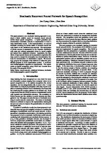
2. APPROXIMATION OF THE NONLINEAR MAPPING F(⋅⋅) USING A RECURRENT NEURAL NETWORK The recurrent neural network used to approximate F(⋅) in (2) consists of three layers; the input layer, the processing layer and the output layer. The input vector is the concatenation of L external inputs, a biased input and delayed signals fed back from the processing layer which consists of N units with bipolar sigmoid activation function. The output layer has a single unit

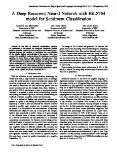
which linearly combines the processing layer outputs. If the network is fully connected, it has a total of N2+(L+1)N connections from the input layer to the processing layer and N connections from the processing layer to the output layer. A RNN predictor with L=2 and N=3 is exhibited in Figure 1. Each delay unit introduces a delay of τN samples. This form of predictor has been extensively studied in [10] for both formant and pitch prediction using the traditional approach. The external inputs were formed by taking p (typically 8-10) successive speech samples for formant prediction and 1-3 samples at a distance equal to the pitch period for pitch prediction. In the context of (2), these predictors are probably suboptimal and require a larger dimension than that is suggested by the embedding theory. The following equations describe the operation of the network: Y(n)=f(WF Y(n-τN)+Wi R(n)) (3) s$(n) = Wo Y(n) (4) where Y(n)=[y1(n),y2(n),⋅⋅⋅yN(n)] is the state vector, R(n)= [1,s(n-1),s(n-τE-1),⋅⋅⋅,s(n-(dE-1)τE-1) is the augmented input vector, Wf is the feedback weight matrix, Wi is the input weight matrix, Wo is the output weight matrix and τN is the network time delay. Adaptation of Wf and Wi is performed using the real-time recurrent learning (RTRL) algorithm [11] and Wo is adapted using the well known LMS algorithm [12]. At the processing layer, being hidden, error signals are not available and they are generated by backpropogating the output error through the linear combiner. ^ s(n)

+

y 3(n) z-τ

N

z-τ

N

z-τ

y2(n)

y1(n)

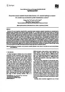
3. COMPARISON OF METHODS WITHIN A UNIFIED FRAMEWORK 3.1 Speech Analysis For a systematic comparison of the approaches introduced above we adopt the framework illustrated in Figure 2 for prediction [13]. The framework consists of two parts; i) The memory unit, ii) The mapping unit. Figure 2. A framework for prediction ^ x(n)

x(n) Memory Unit

Mapping Unit

The success of prediction depends on the following: (a) the amount of information kept in the memory unit relevant to prediction (b) the ability of the mapping unit to realize the actual relation between the information in the memory and the predicted value. Firstly we discuss the amount of past information that can be considered relevant to prediction in the case of speech signals. As is well known, in voiced speech prediction we distinguish between two types of correlations; i) short term correlations and ii) long term correlations. The former indicates the dependency of adjacent samples and the latter is a result of the periodicity in speech signals. The periodicity implies similarity among samples which are one period apart. Therefore, for a successful speech prediction the memory unit should span a time interval of length at least one pitch period.

N

s(n-1) s(n- τE-1)

+1

Figure 1. Proposed Recurrent Neural Network. It is clear that for τN=τE, $ s(n + 1) = F(s(n),s(n - τ E ),L, s(n - (d E - 1)τ E ),L )

(5)

Due to the feedback, the memory of the network is infinite but of fading nature. The authors conjecture that this makes the network more robust to the slightly false estimations of dE. On the other hand, this may allow selection of dE smaller than that required. It is also conjectured that the selection of τN≠τE increases the robustness of the network to the estimation errors in τE by providing interleaved samples that are used in prediction.

Secondly we discuss the structure of the memory in all approaches. For this purpose, we define the memory depth, τD, as the duration of the signal history (in samples) stored in the memory unit and the memory resolution, τR, as the reciprocal of the delay between the signal samples stored in the memory unit. In the traditional prediction approach (equation (1)) the memory unit can be considered as a tapped delay line containing the most recent p speech samples. That is τD=p and τR=1. On the other hand, in the dynamical systems approach (equation (2)) the memory unit consists of dE samples each separated by τE samples. Here, τD=dEτE and τR=1/τE . In the pitch-formant approach, the memory unit is made of two blocks. The first block contains the p most recent speech samples each separated by a unit delay. The second block consists of a few samples around exactly one pitch period away from the predicted sample again each separated by a unit delay. As a result the overall memory depth, τD, is slightly greater than the pitch period and each block has resolution τR=1. We conclude that to meet the requirement (a) mentioned above in the traditional approach (τE=1) we need a relatively large value of p (or dE) depending on the pitch period of the speech

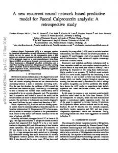
give similar performances in terms of the prediction error. However, in case of linear mapping the prediction performance is expected to be worse when compared to its nonlinear counterparts. -12 -14 -16 -18 MSE (dB)

signal. However, a smaller value of dE is possible in the dynamical systems approach by using a relatively large τE but at the expense of a lower resolution. It appears that, for a given memory depth, the number of samples in the memory unit and the resolution are two conflicting parameters in the sense that our aim is to select dE as small as possible (to avoid the curse of dimensionality), but yet keep the resolution as high as possible (not to miss samples relevant to prediction). In the traditional pitch-formant approach, with the use of two different blocks the resolution is kept high (at least in each block) without sacrificing too much from dimensionality. Since information corresponding to the short and long term correlations is included in the memory unit with a high resolution, that structure is expected to show the best performance as a predictor.

-20 -22 -24 -26

Thirdly we demonstrated the validity of our expectations through some simulations using voiced speech frames taken from male and female speakers. Speech waveforms were lowpass filtered at 3.4 kHz cut-off frequency, sampled at 8 kHz and stored at 16 bits. Each analysis frame consisted of 256 samples. The results were presented for the memory structures with a linear mapping unit by plotting the mean value of the prediction error (MSE) in dB with respect to the memory depth. Figure 3 shows the results corresponding to a female speaker. Here, the pitch period of the analysis frame is 24 samples. The MSE of the pitch-formant approach is shown as a baseline. The so-called formant memory block consists of the most recent 8 samples and the so-called pitch memory block consists of 3 consecutive samples centered at the pitch period. The other two plots are for memory resolutions τR=1 and τR=1/3. The poor performance of the lower resolution and the good performance of the pitch-formant approach are obvious. However, all memory structures have comparable performances when all relevant information is included in the memory as illustrated for τD > pitch period. Finally we extend the discussion to the nonlinear mapping unit and present several experimental results. As mentioned, the possible networks that can be used are MLP, RBF and RNN. The first two are feedforward networks. Being static, they do not contribute to the memory content of the predictor. The RNN, in contrast, has two implicit effects on the memory content: 1) the effective memory depth is increased because of the infinite fading memory (compensates for relatively small dE). 2) the missing samples in the memory are partially supplied by properly selecting the network delay, τN different from the embedding delay,τE (compensates for low resolution). Thus a predictor using an RNN as the mapping unit is expected to outperform the predictors using MLP and RBF in cases where; (i)the memory depth does not cover a full pitch period (ii)the memory depth covers a pitch period but at a low resolution. In other words, for a given performance RNN allows a relatively small dE with a relatively large τE, provided that τN≠τE is properly selected. However, in cases where all relevant information is in the memory unit, we expect all structures to

-28 -30 0

5

10

15

20

25

Memory Depth

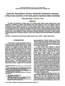
Figure 3. Comparison of different memory structures with the linear mapping unit;female speech. o: τE=1, x: τE=3, _: pitch-formant memory block (p=8, M=3). Figure 4 shows the performances of RNN predictor (with a unity network delay τN=1), MLP predictor and a linear predictor with respect to the memory depth. Note that all of the predictors have memory resolution τR=1. In both RNN and MLP networks the number of neurons was set to 4. In all simulations the learning rate was set to 0.1 and kept fixed and the networks were trained for 1000 epochs. The results were averaged over 10 trials. The performance of the RBF network at comparable complexities was found to be very poor with the learning algorithm that was implemented. So, the RBF network results are not shown to avoid overcrowded plots. In Figure 4 the baseline corresponds to the performance of the pitch-formant RNN [8] with 8 most recent samples and 3 samples around the pitch period. Its better performance at relatively lower complexity (11 input samples) is obvious. Note that the RNN significantly outperforms the MLP network for very short memory depths (1-5 input samples). Their performances becomes comparable as all short term correlated samples are included in the memory. This remains until the implicit memory of RNN starts to capture the samples around the pitch period, though, the external memory depth is still less than the pitch period. Their performances meet again as the external memory covers the full pitch period. Again this behaviour is common to all speech frames. Nevertheless, because of its infinite memory, the RNN outperforms the MLP network if it is not stuck at a local minimum with a relatively bad performance. It is a general belief that learning algorithms in the RNN explores a more complex surface. To check the frequency of occurrence of the above phenomena we run the RNN and the MLP networks over 200 frames of speech taken from 4 speakers. In all simulations τE was chosen as the first minimum of the mutual information function and dE was chosen as the smallest integer greater than the estimated attractor dimension (dE>d+1), even though the estimates are not expected to be accurate due to small size of

analysis frame. The results are presented in Figure 5. Here, the solid line represents the boundary where the performances of the two predictors are equal. Note that the RNN performs better than the MLP for almost all the frames. So, we conclude that it is very safe to use the RNN. -12 -14 -16

MSE (dB)

-18 -20 -22

synthesizer is operated in an autonomous manner by seeding it with an all zero state vector and feeding the output to the delay line which is constructed the same as the memory structure employed in prediction. Here, the fundamental question is “Which predictor implementation is the most suitable for synthesis ?” We claim that the RNN with time delay embedding appears the most promising since it offers a lower dimension for the state space. Lower dimensionality helps a) to avoid curse of dimensionality. b) to decrease the degree of mismatch in the analysis and synthesis models. c) to have a faster convergence to the reconstructed attractor. d) to reduce the computational complexity

-24

-20

-26 -28 -30 -32 0

5

10

15

20

25

30

Memory Depth

Figure 4. Comparison of RNN vs. MLP (N=4, τE=1, τD