a regularized adaptive steplength stochastic approximation scheme

Proceedings of the 2011 Winter Simulation Conference S. Jain, R. R. Creasey, J. Himmelspach, K. P. White, and M. Fu, eds.

A REGULARIZED ADAPTIVE STEPLENGTH STOCHASTIC APPROXIMATION SCHEME FOR MONOTONE STOCHASTIC VARIATIONAL INEQUALITIES

Farzad Yousefian Angelia Nedić Uday V. Shanbhag UIUC, 104 S. Mathews, Urbana, IL 61801, USA ABSTRACT We consider the solution of monotone stochastic variational inequalities and present an adaptive steplength stochastic approximation framework with possibly multivalued mappings. Traditional implementations of SA have been characterized by two challenges. First, convergence of standard SA schemes requires a strongly or strictly monotone single-valued mapping, a requirement that is rarely met. Second, while convergence requires that the steplength sequences need to satisfy ∑k γk = ∞ and ∑k γk2 < ∞, little guidance is provided on a choice of sequences. In fact, standard choices such as γk = 1/k may often perform poorly in practice. Motivated by the minimization of a suitable error bound, a recursive rule for prescribing steplengths is proposed for strongly monotone problems. By introducing a regularization sequence, extensions to merely monotone regimes are proposed. Finally, an iterative smoothing extension is suggested for accommodating multivalued mappings. Preliminary numerical results suggest that the schemes prove effective. 1

INTRODUCTION

In this paper, we consider the solution of a monotone stochastic variational inequality, denoted by VI(X, F), where X ⊆ Rn is a closed and convex set, the ith component of F : X → Rn is defined as Fi (x) , E[ fi (x; ξ )] and f : Rn × Rd → Rn . Note that ξ is a random variable with ξ : Ω → Rd and the associated probability space is denoted by (Ω, F , P). A solution of VI(X, F) is denoted by x∗ where x∗ ∈ SOL(X, F), the solution set of VI(X, F), if (x − x∗ )T F(x∗ ) ≥ 0 for all x ∈ X. It may be recalled that the mapping F(x) is monotone over X if (F(x) − F(y))T (x − y) ≥ 0 for all x, y ∈ X. Variational inequalities (cf. Facchinei and Pang 2003) are a broad class of objects that allows for capturing the set of solutions to convex optimization problems as well as noncooperative Nash games over continuous strategy sets. Stochastic variational inequalities are a relatively less studied class of problems and our interest lies in extensions in which the mapping F comprises of expectations in its components, as examined by Jiang and Xu (2008) and Ravat and Shanbhag (2011). Given that the components of F(x) contains expectations, standard approaches for solving variational inequalities (cf. Facchinei and Pang 2003) cannot be leveraged since this necessitates having analytical expressions for the expectations. Instead, we turn to a simulation-based approach for obtaining solutions. Jiang and Xu (2008) appear to be amongst the first to have analyzed such schemes in the context of strongly monotone stochastic variational inequalities. Extensions to merely monotone regimes have been recently provided by Koshal et al. (2010) where Tikhonov regularization and proximal-point schemes are overlaid on standard SA techniques. One of the motivations for the present work lies in the lack of guidance in choosing steplength sequences; notably, certain choices may lead to significant degradation in performance. Adaptive steplength stochastic approximation procedures have been studied extensively since the earliest work by Robbins and Monro (1951). Subsequently, Kesten (1958) suggested a sequence that adapts to the observed data. Subsequently, under suitable conditions, Sacks (1958) proved that a choice of the form a/k is optimal from the standpoint 978-1-4577-2109-0/11/$26.00 ©2011 IEEE

4115

Yousefian, Nedić, and Shanbhag of minimizing the asymptotic variance. Yet, the challenge lies in estimating the “optimal” a. Subsequently, Venter (1967) in what is possibly amongst the first adaptive steplength SA schemes, considered sequences of the form ak /k where ak is updated by leveraging past information. Averaging techniques were applied by Polyak and Juditsky (1992). More recently, Broadie et al. (2011) consider an adaptive Kiefer-Wolfowitz (KW) SA algorithm and derive upper bounds on its mean-squared error. Yousefian, Nedić, and Shanbhag (2011) presented two adaptive steplength SA schemes for strongly convex programs, both of which produce a sequence of iterates guaranteed to converge almost surely to the true solution. Of these, the first relies on minimizing the upper bound on the error at every step; in fact, such a minimization leads to a recursive rule for updating steplengths and the scheme is referred to as a recursive SA (or RSA) scheme. The second scheme introduces regular reductions in the steplength when a suitable error criterion is satisfied and the associated scheme is referred to as a cascading SA scheme (or CSA) scheme. A random local smoothing approach is employed for accommodating the approximate solution of nonsmooth stochastic convex programs. In this paper, we revisit our RSA scheme with the intent of introducing three key generalizations: (i) First, we extend the regime of applicability of the RSA scheme to strongly monotone stochastic VIs; (ii) Second, we overlay a regularization scheme that facilitates addressing merely monotone stochastic VIs; and (iii) Third, we introduce a smoothing parameter that allows for solving problems with strongly monotone but multivalued maps. The remainder of the paper is organized as follows. In Section 2, we introduce a regularized recursive steplength stochastic approximation scheme for monotone stochastic VIs. We show that this algorithm produces iterates that converge in expectation to the solution. In Section 3, we introduce an iterative smoothing generalization of the recursive scheme. Finally, in Section 4, we present some preliminary numerical results and provide some concluding remarks in Section 5. 2

A REGULARIZED RECURSIVE STEPLENGTH STOCHASTIC APPROXIMATION SCHEME

In Section 2.1, we introduce a regularized SA scheme, akin to that developed by Koshal, Nedić, and Shanbhag (2010). By introducing a recursive rule for updating the steplengths, we present the regularized recursive SA scheme or RRSA scheme in Section 2.2. 2.1 A Regularized Stochastic Approximation scheme Consider a regularized stochastic approximation scheme of the form: xk+1 = ΠX (xk − γk (F(xk ) + ηk xk + wk ))

for all k ≥ 0,

wk = f (xk , ξk ) − F(xk ),

(1)

where {γk } is the stepsize sequence, {ηk } is a nonnegative sequence, and x0 ∈ X is a random initial vector that is independent of the random variable ξ and such that E kx0 k2 < ∞. We make the following two assumptions through our analysis, of which the first pertains to problem parameters and errors and the second to the algorithm parameters (steplength and regularization) sequences. Assumption 1 (a) The sets X ⊂ Rn are closed and convex; (b) with constant L over the set X. F(x) is Lipschitz 2 E kw k2 | F < ∞ almost surely. (c) The stochastic errors wk satisfy ∑∞ γ k k k=0 k Assumption 2 Let the following hold: ηk 2(ηk +L)2

for all k ≥ 0; (b) limk→∞ ηk = 0;

(a)

0 < γk
0 for all k. Then (a)

For all k ≥ 1 we have kyk − yk−1 k ≤ My

(b)

|ηk−1 − ηk | , ηk

where My is a norm bound on the Tikhonov sequence, i.e., kyk k ≤ My for all k ≥ 0. For all k ≥ 1 we have E kxk+1 − yk k2 | Fk ≤ qk (1 + γk ηk )kxk − yk−1 k2 (ηk−1 − ηk )2 1 + qk My ) + γk2 E kwk k2 | Fk , (1 + 2 γk ηk ηk

(2)

(3)

where qk = 1 − 2γk ηk + γk2 (ηk + L)2 . In the remainder of this subsection, we prove convergence of Tikhonov algorithm under weaker assumptions than shown by Koshal et al. (2010). More specifically, we weaken the assumptions limk→∞ ηγkk (ηk + L)2 = 0 and limk→∞ γk ηk = 0 by part (a) of Assumption 2. Proposition 1 Let Assumptions 1 and 2 hold. Also, assume that SOL(X, F) is nonempty. Then, the sequence {xk } generated by iterative Tikhonov scheme (2) converges to the least-norm solution x∗ of VI(X, F) almost surely and for k ≥ 1 we have ηk (ηk−1 − ηk )2 1 2 2 E kxk+1 − yk k2 | Fk ≤ (1 − γk )kxk − yk−1 k2 + qk My2 (1 + ) + γ E kw k | F , (4) k k k 2 γk ηk ηk2 where qk = 1 − 2γk ηk + γk2 (ηk + L)2 . Proof.

From Lemma 2, we have

1 (ηk−1 − ηk )2 (1 + ) + γk2 E kwk k2 | Fk . E kxk+1 − yk k2 | Fk ≤ qk (1 + γk ηk )kxk − yk−1 k2 + qk My 2 γk ηk ηk Next, we estimate the coefficient qk (1 + ηk γk ). From part (a) of Assumption 2 for k ≥ 0 we have (ηk + L)2 1 γk < < 2 ⇒ −2ηk γk + γk2 (ηk + L)2 < 0 ⇒ qk < 1. ηk 2 4117

Yousefian, Nedić, and Shanbhag Therefore, using this and the definition of qk we obtain qk (1 + ηk γk ) = qk + ηk γk qk < qk + ηk γk = 1 − ηk γk + γk2 (ηk + L)2 . Obviously, when 0 < γk
K, and it suffices to examine a shifted sequence. We need to verify that uk and vk satisfy the conditions of Lemma 1 for k ≥ 0. Note that from part (a) of Assumption 2 for k ≥ 0, uk < 1 since for any L > 0, we vk ∞ 2 k have 0 < γk < 2(ηη+L) 2 < η . Assumption 2 (c) implies that ∑k=K uk = ∞. Next, we consider the ratio u k k k and observe that uvkk ≥ 0 for k ≥ 0. We show that its upper bound converges to zero. Since 0 < qk < 1, the ratio uvkk can be bounded as follows 2γk2 2 (ηk−1 − ηk )2 vk 1 ≤ My2 ) + E kwk k2 | Fk (1 + 2 uk ηk γk γk ηk ηk γk ηk 2 2γk 2(ηk−1 − ηk ) 1 )+ E kwk k2 | Fk . = My2 (1 + 3 γk ηk ηk η k γk

(6)

By Assumption 2 (e) and (f), the above two terms converge to zero, implying that limk→∞ uvkk = 0. Finally, by Assumption 1 (c) and Assumption 2 (d), ∑∞ k=K vk < ∞. It follows from Lemma 1 that kxk − yk−1 k converges to zero almost surely. This and the fact that Tikhonov sequence converges to the least-norm solution x∗ of VI(X, F) imply that xk → x∗ almost surely. Remark on choices of γk and ηk : While Assumption 2 appears rather difficult to satisfy, Koshal et al. (2010), show that a stronger form of Assumption 2 is satisfied by γk = k−a and ηk = k−b with a + b < 1 and a > b. We conclude with a corollary that relies on the following assumption on the errors. Assumption 3 The errors wk are such that for some ν > 0 E kwk k2 |Fk ≤ ν 2 a.s. for all k ≥ 0. The following corollary gives a parametric upper bound for the error; this result is applied to obtain the recursive scheme in next part. Corollary 1 Let Assumptions 1, 2, and 3 hold. Also, assume that SOL(X, F) is nonempty. Then, the sequence {xk } generated by iterative Tikhonov scheme (2) converges to the least-norm solution x∗ of V I(X, F) almost surely and for k ≥ 1 we have ηk (ηk−1 − ηk )2 1 (1 + ) + γk2 ν 2 , ∀k ≥ 1, E kxk+1 − yk k2 ≤ (1 − γk )E kxk − yk−1 k2 + qk My2 2 γk ηk ηk2

(7)

where qk = 1 − 2γk ηk + γk2 (ηk + Lk )2 . Proof. The convergence result follows from Proposition 1 while (7) follows from (4) by taking expectations and invoking Assumption 3. 4118

Yousefian, Nedić, and Shanbhag 2.2 A Regularized Recursive Steplength SA Scheme A challenge associated with the implementation of diminishing steplength schemes lies in determining an appropriate sequence {γk }. The key result of this section is the motivation and introduction of a scheme that adaptively updates the steplength across successive iterations; such a rule is derived from the minimization of a suitably defined error function at each step. Let us view the quantity E kxk+1 − yk k2 as an error, denoted by ek+1 , and arising from the use of the stepsize values γ0 , γ1 , . . . , γk . Thus, in the worst case, the error satisfies the following recursive relation for any k ≥ 1: ek+1 (γ1 , . . . , γk ) = (1 −

(ηk−1 − ηk )2 1 ηk γk )ek (γ1 , . . . , γk−1 ) + qk My2 (1 + ) + ν 2 γk2 , 2 2 γk ηk ηk

where qk = 1 − 2γk ηk + γk2 (ηk + Lk )2 , e1 is a positive scalar, ηk is a positive regularization parameter and ν 2 is the upper bound for the second moments of the error norms kwk k. Then, it seems natural to investigate if the stepsizes γ1 , γ1 . . . , γk can be selected so as to minimize the error ek+1 . It turns out that this can indeed be achieved at each iteration. Let us now define the following parameters: (ηk−1 − ηk )2 Mk ηk , ck , −Mk , bk , , ak , , 2 2 ηk ηk (ηk + L)2 dk , Mk fk , Mk (ηk + L)2 + ν 2 . − 2ηk , ηk Mk , My2

(8)

Then, (2.2) may be rewritten as follows for k ≥ 1: ek (γ1 , . . . , γk−1 ) = (1 − ak−1 γk−1 )ek−1 (γ1 , . . . , γk−2 ) +

bk−1 2 + ck−1 + dk−1 γk−1 + fk−1 γk−1 . γk−1

(9)

The presentation of our recursive steplength scheme is significantly simplified by defining a function Dk : R+ → R such that bk 1 − 2 + dk + 2 fk t . (10) Dk (t) , ak t Regularized recursive steplength SA (RRSA) scheme: For k ≥ 1, given an e1 > 0, the RRSA scheme generates a sequence {xk } where xk+1 is updated as per (1), {ηk } satisfies Assumption 2 and γk satisfies D1 (γ1 ) − e1 = 0,

(11)

Dk+1 (γk+1 ) = (1 − ak γk )Dk (γk ) +

bk + ck + dk γk + fk γk 2 . γk

(12)

For k ≥ 1, the above equations lead to a polynomial function of the third degree with respect to γk . We assume that at each iterate, this equation has a positive real root denoted by γk . Furthermore, we often refer to ek (γ1 , . . . , γk−1 ) by ek whenever this is unambiguous. In our main result of this subsection, we show k that the stepsizes γi , i = 1, . . . , k − 1, minimize the errors ek over the range that 0 < γk < 2(ηη+L) 2 for k ≥ 1, k where L is the Lipschitz constant associated with the mapping F(x). Proposition 2 Let ek (γ1 , . . . , γk−1 ) be defined as in (2.2), where e1 > 0 is such that (11) has a real positive root as γ1∗ , and we assume that for each k ≥ 1, equation (12) has a real positive root as γk∗ . Let the sequence {γk∗ } be given by (11)–(12). Suppose that the sequence {ηk }∞ k=0 is nonincreasing and fixed. Then, the following hold: (a)

∗ )= The error ek satisfies ek (γ1∗ , . . . , γk−1 are defined in (8).

bk 2 ηk (− γ ∗ 2 k

4119

+ dk + 2 fk γk∗ ) for all k ≥ 1, where bk , dk , and fk

Yousefian, Nedić, and Shanbhag (b)

For each k ≥ 1, the vector (γ1∗ , γ1∗ , . . . , γk∗ ) minimizes ek+1 (γ1 , . . . , γk ) over the set ηj k Gk , α ∈ R : 0 < α j < for j = 1, . . . , k . 2(η j + L)2 Additionally, for any k ≥ 2 and any (γ1 , . . . , γk−1 ) ∈ Gk−1 , we have ! b k ∗ ek (γ1 , . . . , γk−1 ) − ek (γ1∗ , . . . , γk−1 )≥ + fk (γk − γk∗ )2 ≥ 0. γk∗ 2 γk

Proof. (a) We use induction on k to prove our result. Note that the result holds trivially for k = 1 from ∗ ) = 1 (− bk + d + 2 f γ ∗ ) for (11) and definition of function D1 . Next, assume that we have ek (γ1∗ , . . . , γk−1 k k k ak γk∗ some k, and consider the case for k + 1. By the definition of the error ek in (2.2), we have ∗ ek+1 (γ1∗ , . . . , γk∗ ) = (1 − ak γk∗ )ek (γ1∗ , . . . , γk−1 )+

bk + ck + dk γk∗ + fk γk∗ 2 γk∗

bk + ck + dk γk∗ + fk γk∗ 2 γk∗ bk+1 1 ∗ ∗ (− ∗ 2 + dk+1 + 2 fk+1 γk+1 = Dk+1 (γk+1 ), )= ak+1 γk+1 = (1 − ak γk∗ )Dk (γk∗ ) +

where the second equality follows by the inductive hypothesis and definition of Dk in (10), the third inequality follows by (12), and the last inequality follows by definition of Dk+1 in (10). ∗ ) minimizes the error e for all k ≥ 2. We again use mathematical (b) We now show that (γ1∗ , γ2∗ , . . . , γk−1 k induction on k. By the definition of the error e2 , we have e2 (γ1 ) − e2 (γ1∗ ) = (1 − a1 γ1 )e1 +

b1 b1 + c1 + d1 γ1 + f1 γ12 − (1 − a1 γ1∗ )e1 − ∗ − c1 − d1 γ1∗ − f1 γ1∗ 2 . γ1 γ1

Using (11) and definition of D1 in (10) we have 1 b1 1 1 )(− ∗ + d1 + 2 f1 γ1∗ ) + b1 ( − ∗ ) + d1 (γ1 − γ1∗ ) + f1 (γ12 − γ1∗ 2 ) a1 γ1 γ1 γ1 b1 1 b1 1 = − ∗ + d1 γ1∗ + 2 f1 γ1∗ 2 + ∗ 2 γ1 − d1 γ1 − 2 f1 γ1∗ γ1 + b1 ( − ∗ ) + d1 (γ1 − γ1∗ ) + f1 (γ12 − γ1∗ 2 ) γ1 γ1 γ1 γ1

e2 (γ1 ) − e2 (γ1∗ ) = a1 (γ1∗ − γ1 )(

= b1 (1 −

γ1 1 1 b1 (γ1∗ − γ1 )2 2 ∗2 ∗ )( − ) + f (γ + γ − 2γ γ ) = + f1 (γ1 − γ1∗ )2 ≥ 0, 1 1 1 1 1 γ1∗ γ1 γ1∗ γ1∗ 2 γ1

where the last inequality follows by positiveness of b1 and f1 . Now suppose that ek (γ1 , . . . , γk−1 ) ≥ ∗ ) holds for some k and any (γ , . . . , γ ek (γ1∗ , . . . , γk−1 1 k−1 ) ∈ Gk . We want to show that ek+1 (γ1 , . . . , γk ) ≥ ∗ ek+1 (γ1 , . . . , γk∗ ) holds as well for all (γ1 , . . . , γk ) ∈ Gk+1 . To simplify the notation we use e∗k+1 to denote the error ek+1 evaluated at (γ1∗ , γ1∗ , . . . , γk∗ ), and ek+1 when evaluating at an arbitrary vector (γ1 , γ1 , . . . , γk ) ∈ Gk+1 . Using (2.2) we have bk bk + ck + dk γk + fk γk2 − (1 − ak γk∗ )e∗k − ∗ − ck − dk γk∗ − fk γk∗ 2 γk γk b bk k ≥ (1 − ak γk )e∗k + + ck + dk γk + fk γk2 − (1 − ak γk∗ )e∗k − ∗ − ck − dk γk∗ − fk γk∗ 2 γk γk

ek+1 − e∗k+1 = (1 − ak γk )ek +

4120

Yousefian, Nedić, and Shanbhag where the last inequality follows by the induction hypothesis and the observation that (1 − ak γk ) > 0 from the feasibility of the sequence {γ j }kj=1 with respect to Gk . Using (12) and the definition of Dk in (10), 1 bk 1 1 )(− ∗ + dk + 2 fk γk∗ ) + bk ( − ∗ ) + dk (γk − γk∗ ) + fk (γk2 − γk∗ 2 ) ak γk γk γk bk 1 bk 1 = − ∗ + dk γk∗ + 2 fk γk∗ 2 + ∗ 2 γk − dk γk − 2 fk γk∗ γk + bk ( − ∗ ) + dk (γk − γk∗ ) + fk (γk2 − γk∗ 2 ) γk γk γk γk

ek+1 − e∗k+1 = ak (γk∗ − γk )(

= bk (1 −

bk (γk∗ − γk )2 1 γk 1 ∗ 2 ∗2 + fk (γk − γk∗ )2 ≥ 0, − 2γ γ ) = )( − ) + f (γ + γ k k k k k γk∗ γk γk∗ γk∗ 2 γk

where the last inequality follows by positiveness of bk and fk . Hence, we have ek (γ1 , . . . , γk−1 ) − ∗ ) ≥ ν 2 (γ − γ ∗ )2 for all k ≥ 2 and all (γ , . . . , γ ek (γ1∗ , . . . , γk−1 1 k−1 ) ∈ Gk . Therefore, for all k ≥ 2, the k k vector (γ1 , . . . , γk−1 ) ∈ Gk is a minimizer of the error ek . 2.3 Convergence of RRSA Scheme In this part, we show that the RRSA scheme converges in expectation to the solution for a fixed choice of regularization sequence by employing the following result proved by Koshal et al. (2010). Proposition 3 Let Assumptions 1(a)-(b), and 3 hold and suppose that SOL(X, F) is nonempty. Consider the choice ηk = k−b and γk = k−a for all k, where a, b ∈ (0, 1), a + b < 1, and a > b. Then, this choice satisfies Assumptions 1(c), and 2 and the sequence {xk } generated by iterative Tikhonov scheme (2) converges to the least-norm solution x∗ of VI(X, F) almost surely. Proposition 4 Let Assumptions 1(a)-(b), and 3 hold and suppose that SOL(X, F) is nonempty. Consider the choice ηk = k−b for all k, where b ∈ (0, 1/2) and suppose that {γk∗ }∞ k=1 is given by the adaptive scheme (11)-(12). Then, the sequence {xk } generated by iterative Tikhonov scheme (2) converges in expectation to the least-norm solution x∗ of VI(X, F). Proof. Let γ¯k = k−a for all k, where a + b < 1 and b < a. Now suppose that {x¯k } is generated by the iterative Tikhonov scheme (2) with {γ¯k } and {ηk }. Then from Lemma 3, Assumptions 1(c), and 2 are satisfied by this choice of {ηk } and {γ¯k } and therefore by Proposition 1, E kx¯k+1 − yk k2 goes to zero where {yk } is the sequence of exact solution to V I(X, F + ηk I) for k ≥ 0. This implies that the upper bound sequence defined by (2.2) goes to zero. Now, from Proposition 2(b), we know that for the sequence {xk } generated by the iterative Tikhonov scheme (2) with {γk∗ } and {ηk } the following inequality holds for k ≥ 0: ∗ ek (γ1 , . . . , γk−1 ) − ek (γ1∗ , . . . , γk−1 ) ≥ 0.

(13)

Since E kx¯k+1 − yk k2 − E kxk+1 − yk k2 ≥ 0 and by noting that E kx¯k+1 − yk k2 → 0 when k goes to infinity, we conclude that the sequence {xk } generated by the RRSA scheme converges in expectation to the least-norm solution x∗ of VI(X, F). Remark on almost-sure convergence: It is worth noting that almost-sure convergence of the estimators may be proved by showing that the sequence {γk } satisfies the requirements of Lemma 1. This requires a deeper analysis of the roots and will not be pursued further, given the size restrictions of this paper. 3

AN ITERATIVE SMOOTHING RECURSIVE SA SCHEME

Yousefian, Nedić, and Shanbhag (2011) considered stochastic optimization problems with nonsmooth integrands and inspired by Lakshmanan and Farias (2008), employed a random local smoothing of the objective in constructing a stochastic approximation scheme. In fact, a more extensive study of the literature 4121

Yousefian, Nedić, and Shanbhag revealed that such smoothing techniques had been employed extensively in the past and were referred to as Steklov-Sobolev smoothing techniques. Succinctly, such smoothing approaches led to an approximation that was shown to admit Lipschitzian properties. In fact, the growth rate (with problem size) of the Lipschitz constant associated with the gradient of the objective may be quantified under different types of smoothing distributions, as derived by Yousefian, Nedić, and Shanbhag (2011) and Lakshmanan and Farias (2008). In this section, we make two extensions to our earlier work. First, we extend the approach to address stochastic variational inequalities which may arise from either stochastic optimization problems or Nash games. Second, while our earlier approach obtained an approximate solution since a small, but fixed, smoothing parameter was employed, we consider how this smoothing parameter may be reduced after every iteration, leading to an iterative smoothing scheme, with the intent of obtaining the true solution. For purposes of simplicity, we assume that the original mapping is strongly monotone, implying that there is no need for employing a regularization term. 3.1 Nonsmooth Stochastic Optimization Problems and Nash games We motivate our approach by considering a nonsmooth stochastic Nash game. Consider an N−player Nash game in which the ith player solves the following problem, given x−i , (x j )i6= j∈{1,...,N} : Ag(x−i )

min

xi ∈Xi

E[ fi (xi ; x−i , ξ )] ,

(14)

where for i = 1, . . . , N, Xi ⊆ Rni is a closed and convex set, ∑Ni=1 ni = n and fi : Rn × Ω → R is a continuous convex function for all x−i ∈ ∏ j6=i X j . Recall that a Nash equilibrium is given by a tuple {xi∗ }Ni=1 such that xi∗ ∗ ) for i = 1, . . . , N. Then the resulting Nash equilibrium is given by a solution to a multi-valued solves Ag(x−i variational inequality VI(X, ∂ F) where X , ∏Ni=1 Xi and ∂ F(x) , ∂xi E[ fi (x; ξ )] for i = 1, . . . , N. Note that if fi (x; ξ ) is differentiable in xi , given x−i , VI(X, ∂ F) reduces to VI(X, F) where F(x) = (∇xi E[ fi (x; ξ )])Ni=1 is a single-valued mapping. Clearly, if N = 1, then this game reduces to a stochastic optimization problem. 3.2 An Iterative Smoothing Extension of the RSA Scheme Consider a smoothed approximation of the stochastic Nash game in which the ith player solves the following smoothed problem: min

xi ∈Xi

E[E[ fi (xi + zi ; x−i , ξ ) | ξ ]] ,

(15)

where the inner expectation is with respect to zi ∈ Rni , a random vector with a compact support. Then z , (zi )Ni=1 ∈ Rn is an n−dimensional random vector with a probability distribution over the n-dimensional ball centered at the origin and with radius ε. If fî is defined as fî , E{ fi (xi + zi ; x−i ; ξ ) | ξ }, then ˆ F(x) , (∇xi fî )Ni=1 . For the mapping Fˆ to be well defined, we need to enlarge the underlying set X so that the mapping F(x + z) is defined for every x ∈ X. In particular, for a set X ⊆ Rn and ε > 0, we let Xε be the set defined by Xε = {y | y = x + z, x ∈ X, z ∈ Rn , kzk ≤ ε}. We employ a uniform distribution for purposes of smoothing but a normal distribution may also work, as considered by Lakshmanan and Farias (2008). However, distributions with finite support seem more appropriate for capturing local behavior of a function, as well as to deal with the problems where the function itself has a restricted domain. Our choice lends itself readily for computation of the resulting Lipschitz constant and for assessment of the growth of the Lipschitz constant with the size of the problem. Suppose z ∈ Rn is a random vector with uniform distribution over the n-dimensional ball centered at the origin and with a radius ε, i.e., z has the following probability density function:  1  cn ε n for kzk ≤ ε, (16) pu (z; ε) =  0 otherwise, 4122

Yousefian, Nedić, and Shanbhag n

π2 where cn = n and Γ is the gamma function given by Γ( 2 + 1)  n if n is even, n  2 ! Γ +1 =  √ 2 n!! π 2(n+1)/2 if n is odd, where !! is the double factorial symbol. We consider a stochastic approximation scheme in which the parameter specifying the size of the support of the smoothing distribution is reduced after every iteration: ˆ k ) + wk ) xk+1 = ΠX xk − γk (F(x for all k ≥ 0, N

ˆ k ), wk = sk − F(x

where sk ∈ ∏ ∂xi fi (xi + zki ; x−i , ξ ), i=1

where zk is drawn from a uniform distribution pu (z; εk ) and εk → 0. In effect, the step computation is modified by a randomness drawn from a uniform distribution with steadily decreasing support. While this seems intuitive form the standpoint of recovering convergence, the rate at which εk is reduced remains crucial from the standpoint of recovering convergence. Yousefian, Nedić, and Shanbhag (2011) derive a growth property for the Lipschitz constant associated with the smoothed gradient of the optimization problem; in particular, we show that the Lipschitz constant is of the form n!! C ˆ ˆ kx − yk for all x, y ∈ X, kF(x) − F(y)k ≤ κ (n − 1)!! ε where κ = π2 if n is even and κ = 1 otherwise. Therefore, as ε → 0, the Lipschitz constant grows to infinity. Yet, if this growth rate is sufficiently small, one may recover almost-sure convergence. The crux of the proof lies in showing that the recursive steplength rule is feasible with respect to the Lipschitz constants which η are growing in each step. More specifically, Gk requires that 0 < γ j < 2(η+L(ε 2 for j = 1, . . . , k. Under j )) this modified specification of Gk , the optimality of the steplength choices would need to be established. Almost-sure convergence follows if this steplength sequence satisfies ∑k γk2 < ∞ and ∑k γk = ∞; verifying these requirements is a focus of ongoing research. 4

NUMERICAL RESULTS

In this section, we present some preliminary numerical results detailing the performance of the proposed schemes. In Section 4.1, we consider a stochastic network utility problem and compare the performance of the proposed RRSA scheme with an ITR scheme and a standard SA implementation with stepsizes given by γk = 1/k. A sensitivity analysis is also conducted for different values of problem parameters in an effort to gauge the stability of the performance of each scheme. Nonsmooth stochastic variational problems are examined in Section 4.2 where an iterative smoothing counterpart of the RSA scheme is examined. Note that the computational results were developed on Matlab 7.0 on a Linux OS. Furthermore, the true solutions were computed by solving a sample-average approximation (SAA) problem. 4.1 A Stochastic Network Utility Problem We consider a spatial network with n users competing over L1 links. Suppose the ith user’s utility function is denoted by ξi log(1 + xi ). Additionally, a congestion cost is imposed on every user of the form c(x) = kAxk2 where A is defined as the adjacency matrix with binary elements that specifies the set of links traversed by the traffic generated by a particular user. We assume that the user traffic rates are restricted by capacity constraints ∑ni=1 Ali xi ≤ Cl for every link l where Cl is the aggregate traffic through link l. The resulting equilibrium conditions are given by a stochastic monotone variational inequality. 4123

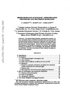
Yousefian, Nedić, and Shanbhag Employing the same starting point, we generate 100 replications for each scheme and compare the average error norm with respect to the reference solution as computed from the solution of an SAA problem. Figure 1 shows the trajectory of the mean error for the ITR, RRSA, and HSA schemes. Note that the x−axis denotes the iteration number while the y−axis denotes the logarithm of the averaged error over a 100 replications. In other words, for a fixed problem and a fixed scheme, we run the simulation 100 times and averaged the terms kxk − x∗ k where x∗ is the solution of VI(X, F) from solving an SAA problem and 1 ≤ k ≤ N. Here, we assume that C1 = (0.10, 0.15, 0.20, 0.10, 0.15, 0.20, 0.20, 0.15, 0.25) = 0.1C2 = 0.01C3 and x is constrained to be nonnegative. We also assume that ξi is a uniform random variable between zero and β for any i where β is a positive parameter. Table 1 displays the 90% confidence intervals for nine parameter settings, categorized into three groups. In the first group, the sensitivity of the results to changing N is examined while the second and third groups investigate the impact of changing β and C. Insights: We observe that the adaptive scheme performs favorably in comparison with the other two schemes from several standpoints. From Figure 1, we observe that the RRSA scheme tends to perform well across three different problem settings while the performance of a standard SA implementation is characterized by tremendous variability. In fact, as seen in Figures 1a and 1b, the HSA scheme performs poorly. It should be emphasized that the standard HSA scheme is not guaranteed to converge for merely monotone variational problems but is often a de-facto choice in simulation-based optimization. Furthermore, when HSA does outperform RRSA (as in Figure 1c), it does not contradict the optimality of adaptive stepsizes since the HSA scheme is not part of the feasible set of sequences that RRSA is optimized over. Table 1 shows the sensitivity of the three schemes to changes in parameters. One can immediately see that the RRSA scheme produces iterates with lower average error and is relatively robust to parametric changes. The HSA scheme, on the contrary, is extremely sensitive to such modifications, particularly when they arise in the form of a change in β .

(a) β = 5, C = C1

(b) β = 10, C = C1

(c) β = 10, C = C3

Figure 1: Trajectories of average error for the stochastic network utility problem. Table 1: Parametric Sensitivity of Confidence Intervals. N

β

C

P(i) 1 2 3 4 5 6 7 8 9

N 4000 2000 1000 4000 4000 4000 4000 4000 4000

β 5 5 5 10 10 10 20 50 100

C C1 C1 C1 C1 C2 C3 C1 C1 C1

ITR - 90% CI [4.34e−2,5.05e−2] [5.93e−2,6.99e−2] [9.58e−2,1.11e−1] [9.79e−2,1.16e−1] [9.79e−2,1.16e−1] [9.79e−2,1.16e−1] [2.88e−1,3.23e−1] [1.83e−1,1.91e−1] [4.62e−0,4.75e−0]

4124

RRSA - 90% CI [1.10e−2,1.32e−2] [1.45e−2,1.71e−2] [1.64e−2,1.93e−2] [1.44e−2,1.71e−2] [1.53e−2,1.82e−2] [1.88e−2,2.23e−2] [1.87e−2,2.22e−2] [2.75e−2,3.25e−2] [3.85e−2,4.48e−2]

HSA - 90% CI [5.01e−1,6.69e−1] [6.09e−1,7.93e−1] [7.31e−1,9.30e−1] [2.52e−0,3.04e−0] [5.10e−3,6.30e−3] [5.10e−3,6.30e−3] [7.30e−0,8.50e−0] [2.25e+1,2.57e+1] [4.80e+1,5.45e+1]

Yousefian, Nedić, and Shanbhag 4.2 A Nonsmooth Stochastic Optimization Problem Next, we examine the following nonsmooth optimization problem: ) ( " !# n η i 2 + kxk , + ξi xi min f (x) = E φ ∑ x∈X 2 i=1 n

(17)

where X = {x ∈ Rn |x ≥ 0, ∑ni=1 xi = 1} and ξi are independent and identically distributed random variables with mean zero and variance one for i = 1, . . . , n. The function φ (·) is a piecewise linear convex function given by φ (t) = max1≤i≤m {vi + sit}, where vi and si are constants between zero and one, and f (x, ξ ) = φ (∑ni=1 ( ni + ξi )xi )). By applying our smoothing approach, the modified problem is given by ( " #) n i η min fˆ(x) , E φ ( ∑ ( + ξi )(xi + zi )) + kx + zk2 , (18) x∈X 2 i=1 n where z ∈ Rn is the uniform distribution on a ball with radius ε with independent elements zi , 1 ≤ i ≤ n. While space limitations preclude a detailed numerical study, we provide schematics of the performance of our iterative smoothing extension of the RSA scheme in Figure 2 for two problem instances in which the √ smoothing parameter is reduced at 1/k and 1/ k, of which the former displays better properties.

√ (b) n = 5, εk = 1/ k

(a) n = 10, εk = 1/k

Figure 2: The stochastic utility problem: random smoothing with adaptive stepsizes.

5

CONCLUDING REMARKS

Traditionally, a key challenge in the implementation of SA schemes lies in the choice of the steplength sequences. In earlier work in the context of stochastic convex optimization, we developed a simple recursive procedure that was sensitive to problem parameters but relied on strong convexity. We extend this regularized recursive SA scheme to the regime of merely monotone stochastic variational inequalities by overlaying a regularization parameter that is reduced after every gradient step. Convergence in mean of the associated sequence is presented. The second part of the paper introduces an iterative smoothing generalization that allows for multivalued mappings. Preliminary results on a class of stochastic convex and nonsmooth problems suggest that adaptive schemes perform well in comparison with standard implementations. REFERENCES Broadie, M., D. Cicek, and A. Zeevi. 2011. “General Bounds and Finite-Time Improvement for the Kiefer-Wolfowitz Stochastic Approximation Algorithm”. Operations Research (To appear). Facchinei, F., and J.-S. Pang. 2003. Finite-dimensional variational inequalities and complementarity problems. Vols. I,II. Springer Series in Operations Research. New York: Springer-Verlag.

4125

Yousefian, Nedić, and Shanbhag Jiang, H., and H. Xu. 2008. “Stochastic approximation approaches to the stochastic variational inequality problem”. IEEE Transactions on Automatic Control 53 (6): 1462–1475. Kesten, H. 1958. “Accelerated stochastic approximation”. Ann. Math. Statist 29:41–59. Koshal, J., A. Nedić, and U. V. Shanbhag. 2010. “Single Timescale Regularized Stochastic Approximation Schemes for Monotone Nash games under Uncertainty”. Proceedings of the IEEE Conference on Decision and Control (CDC):231–236. Lakshmanan, H., and D. Farias. 2008. “Decentralized Recourse Allocation In Dynamic Networks of Agents”. SIAM Journal on Optimization 19 (2): 911–940. Polyak, B. 1987. Introduction to optimization. New York: Optimization Software, Inc. Polyak, B., and A. Juditsky. 1992. “Acceleration of stochastic approximation by averaging”. SIAM J. Control Optim. 30 (4): 838–855. Ravat, U., and U. V. Shanbhag. 2011. “On the Characterization of Solution Sets in Smooth and Nonsmooth Convex Stochastic Nash Games”. SIAM Journal of Optimization (To appear). Robbins, H., and S. Monro. 1951. “A stochastic approximation method”. Ann. Math. Statistics 22:400–407. Sacks, J. 1958. “Asymptotic distribution of stochastic approximation procedures”. Ann. Math. Statist. 29:373– 405. Venter, J. H. 1967. “An extension of the Robbins-Monro procedure”. Ann. Math. Statist. 38:181–190. Yousefian, F., A. Nedić, and U. Shanbhag. 2011. “On Stochastic Gradient and Subgradient Methods with Adaptive Steplength Sequences”. Automatica (To appear). AUTHOR BIOGRAPHIES FARZAD YOUSEFIAN received his B.S. degree in 2006, and M.S. degree in 2008, from Sharif University of Technology, both in Industrial Engineering. He has been in the Ph.D. program at the Department of Industrial and Enterprise Systems Engineering, University of Illinois at Urbana-Champaign since 2008. His current research interests lie in the development of algorithms in the regime of variational inequalities and optimization in uncertain and nonsmooth settings. ´ received her B.S. degree from the University of Montenegro (1987) and M.S. degree ANGELIA NEDIC from the University of Belgrade (1990), both in Mathematics. She received her Ph.D. degrees from Moscow State University (1994) in Mathematics and Mathematical Physics, and from Massachusetts Institute of Technology in Electrical Engineering and Computer Science (2002). She has been at the BAE Systems Advanced Information Technology from 2002-2006. Since 2006 she is an Assistant professor at the Department of Industrial and Enterprise Systems Engineering, University of Illinois at Urbana-Champaign. Her general interest is in optimization including fundamental theory, models, algorithms, and applications. Her current research interest is focused on large-scale convex optimization, distributed multi-agent optimization, and duality theory with applications in decentralized optimization. She received an NSF Faculty Early Career Development (CAREER) Award in 2008 in Operations Research. UDAY V. SHANBHAG received his Ph.D. degree in operations research from the Department of Management Science and Engineering, Stanford University, Stanford, CA, in 2006. He also holds a Bachelors degree from the Indian Institute of Technology (IIT), Bombay (1993) and masters degrees from the Massachusetts Institute of Technology (MIT), Cambridge (1998). He is currently an Assistant Professor in industrial and enterprise systems engineering at the University of Illinois at Urbana-Champaign and his interests lies in the development of analytical and algorithmic tools in the context of optimization and variational problems, in regimes complicated by uncertainty, dynamics and nonsmoothness. Dr. Shanbhag received the triennial A.W. Tucker Prize for his dissertation from the mathematical programming society (MPS) in 2006 and the Computational Optimization and Applications (COAP) Best Paper Award in 2007 (with Walter Murray).

4126