The Robinson-Foulds (RF) metric is the measure most widely used in comparing .... Consider an m à NB matrix V in which we want to compute the ·2-norm be- ..... Hillis, D., Heath, T., St John, K.: Analysis and visualization of tree space. Syst.
A Sublinear-Time Randomized Approximation Scheme for the Robinson-Foulds Metric Nicholas D. Pattengale and Bernard M.E. Moret Department of Computer Science, University of New Mexico, Albuquerque, NM 87131, USA {nickp, moret}@cs.unm.edu
Abstract. The Robinson-Foulds (RF) metric is the measure most widely used in comparing phylogenetic trees; it can be computed in linear time using Day’s algorithm. When faced with the need to compare large numbers of large trees, however, even linear time becomes prohibitive. We present a randomized approximation scheme that provides, with high probability, a (1 + ε) approximation of the true RF metric for all pairs of trees in a given collection. Our approach is to use a sublinear-space embedding of the trees, combined with an application of the Johnson-Lindenstrauss lemma to approximate vector norms very rapidly. We discuss the consequences of various parameter choices (in the embedding and in the approximation requirements). We also implemented our algorithm as a Java class that can easily be combined with popular packages such as Mesquite; in consequence, we present experimental results illustrating the precision and running-time tradeoffs as well as demonstrating the speed of our approach.
1 Introduction The need to compare phylogenetic trees is common. Many reconstruction methods (particularly maximum parsimony and Bayesian methods) produce a large number of possible trees. Trees are also built for the same collection of organisms from different types of data (e.g., nucleotide or codon sequences for one or more genes, gene-order data, protein folds, but also metabolic and morphological data). Phylogenetic trees can be compared and the result summarized in many ways; for instance, consensus methods [1] return a single tree that best summarizes the information present in the entire collection, while supertree methods (typically used when the trees are built on different, overlapping subsets of organisms) [2] combine the individual trees into a single larger one. A more elementary step is to produce estimates of how much the trees differ from each other, by computing pairwise similarity or distance measures. Here again, many approaches have been used, such as computing pairwise edit distances based on tree rearrangement operators [3, 4]; the most common distance measure between two trees, however, is the Robinson-Foulds (RF) metric [5]. This measure is in widespread use because it can be computed in linear time [6], is based directly on the edge structure of the trees and their induced bipartitions, and is a lower bound on the more expensive edit distances. Yet, as the size of datasets used by researchers grows ever larger, even a linear-time computation of pairwise distances becomes onerous. A. Apostolico et al. (Eds.): RECOMB 2006, LNBI 3909, pp. 221–230, 2006. c Springer-Verlag Berlin Heidelberg 2006 �
222
N.D. Pattengale and B.M.E. Moret
In this paper, we present the first sublinear-time algorithm to compute pairwise RF distances among a collection of trees. Our algorithm is a randomized approximation scheme: it returns, with high probability, an approximation that is guaranteed to be within (1 + ε) of the true distance, where ε > 0 can be chosen arbitrarily small. Our approach uses a sublinear-space embedding of the trees, combined with an application of the Johnson-Lindenstrauss lemma [7] to approximate vector norms rapidly. We discuss the consequences of various parameter choices (in the embedding and in the approximation requirements). We also implemented our algorithm as a Java class that can easily be combined with popular packages such as Mesquite [8]; in consequence, we present experimental results illustrating the precision and running-time tradeoffs as well as demonstrating the speed of our approach.
2 Terminology and Definitions A phylogenetic tree is an undirected, connected, acyclic graph; its leaves (also called tips) correspond to the taxa about which data was collected, while its internal nodes all have degree at least 3. If every internal node of a phylogenetic tree has degree equal to 3, the tree is said to be binary or fully resolved. We will use Tn to denote a set of phylogenetic trees on n taxa. Removing an edge (a, b) from a tree T disconnects the tree, creating two smaller trees, Ta (containing a) and Tb (containing b). Note that a (resp., b) might now have only degree 2 in Ta (resp., Tb ), in which case we remove it (connecting its two neighbors directly to each other) in order to preserve the constraint that each internal node have degree at least 3. Cutting T into Ta and Tb induces a bipartition (or split) of the set S of taxa of T into the set A of taxa of Ta and the set B of taxa of Tb , a bipartition that we denote A|B. Thus there exists a one-to-one correspondence between the bipartitions of S and the edges of T , so that each tree is uniquely characterized by the set of bipartitions it induces. If S has n taxa, then any (unrooted) phylogenetic tree for S has at most 2n − 3 edges and so induces at most 2n − 3 bipartitions, only a small subset of the � n2 � �
NB =
∑
i=1
� n ≈ 2n−1 i
possible bipartitions of the set S. Moreover, n of these bipartitions are trivial bipartitions that split S into a one-element set against the remaining n − 1 elements—trivial, because these n bipartitions are common to all phylogenetic trees on S and thus need not be explicitly recorded. We shall denote by B(T ) the set of (at most n − 3) nontrivial bipartitions of S induced by T . The Robinson-Foulds distance [5] between two trees on the same set S of taxa is simply a normalized count of the bipartitions induced by one tree, but not by the other. Definition 1. Given a set S of taxa and two phylogenetic trees, T1 and T2 , on S, the Robinson-Foulds distance between T1 and T2 is RF(T1 , T2 ) =
1 (|B(T1 ) − B(T2)| + |B(T2 ) − B(T1)|) 2
A Sublinear-Time Randomized Approximation Scheme for the RF Metric
223
This measure of dissimilarity is easily seen to be a metric [5] and can be computed in linear time [6]. We mentioned that one could also define edit distances between trees, in the context of one or more operators that alter the structure of a tree. Two commonly used operators are the Nearest Neighbor Interchange (NNI) and the more powerful Tree Bisection and Reconnection (TBR)—see [4, 9] for definitions and discussions of these operators. Applying the NNI operator to T1 can change RF(T1 , T2 ) by at most 1, while applying the TBR operator to T1 can change RF(T1 , T2 ) almost arbitrarily. We use these operators in generating test sets for our RF approximation routine, as discussed in Section 5.
3 Theoretical Basis for the Algorithm The key concept in our approach is representation. Our approximation algorithm is a reduction to the computation of vector norms in a suitable vector space and the sublinear running time results from our ability to represent the necessary characteristics of phylogenetic trees in sublinear space. More specifically, we represent phylogenetic trees as vectors in such a way that RF distances become simply the � · �1 -norm of the difference vector, then generalize the result to arbitrary � · � p -norms for p ≥ 1.1 We then borrow a technique from high-dimensional geometry to reduce the dimensionality of tree vectors while maintaining pairwise � · �2-norms. Finally we combine these techniques to obtain a fast approximation algorithm for computing RF distances. 3.1 Bit-Vector Representation
Ë
Consider a (bijective) function f : T ∈Tn B(T ) → IN that assigns a unique integer in the interval [1, NB] (recall that NB is the number of possible bipartitions of the set) to each bipartition. Definition 2. The bit-vector representation of a phylogenetic tree T is vT ∈ IRb where we have � 1 f −1 (i) ∈ T vT [i] = 0 otherwise Obviously, this representation is quite space-consuming and proportionally timeconsuming to produce; fortunately, we need only consider the bits set to 1, as discussed in Section 4.2. By construction the �.�1 -norm between tree vectors is the (non-normalized) RF distance. Theorem 1. ∀T1 , T2 ∈ Tn , RF(T1 , T2 ) = 12 �vT1 − vT2 �1 . Proof. For all s ∈ B(T1 ) − B(T2) (resp., B(T2 ) − B(T1)), we have vT1 [ f (s)] = 1 (resp., vT2 [ f (s)] = 1) and vT2 [ f (s)] = 0 (resp., vT2 [ f (s)] = 0). For all s ∈ B(T1 ) ∩ B(T2 ), we also Ë have vT1 = vT2 = 1 and, for all s ∈ T ∈Tn B(T ) − (B(T1 ) ∪ B(T2 )), we have vT1 = vT2 = 0. Thus we can conclude �vT1 − vT2 �1 = |B(T1 ) − B(T2 )| + |B(T2 ) − B(T1 )| = 2 · RF(T1 , T2 ) 1
� �1 The � · � p -norm of a vector v = (v1 v2 . . . vk ) is �v� p = ∑ki=1 |vi | p p .
224
N.D. Pattengale and B.M.E. Moret
3.2 Properties of � · � p-Norms of Bit-Vectors Theorem 2. For an arbitrary vector v ∈ IRb where every element is chosen from the set {−k, 0, k} (for arbitrary k > 0), we have �v�1 = k1−p · (�v� p) p . Proof. Assume that v has c entries of value ±k; we can write �
b
∑ (|vi |)
�v� p =
� 1p p
1
1
= (ck p ) p = c p k
i=1 b
�v�1 = ∑ |vi | = ck = c
p−1 p
1
(c p k) = c
p−1 p
�v� p
i=1
Raising the first result to the power (p − 1) and solving for c c
p−1 p
p−1 p
yields
= k1−p · (�v� p) p−1
and substituting into the second result finally yields �v�1 = k1−p · (�v� p) p
Corollary 1. For bit-vectors (k = 1) we have �v�1 = (�v� p ) p ; in particular, we have �v�1 = (�v�2 )2 . 3.3 Reducing Dimensionality We briefly outline a result of Johnson and Lindenstrauss [7] for norm-preserving embeddings; see [10, 11, 12] for a more detailed treatment and proofs. Consider an m × NB matrix V in which we want to compute the � · �2 -norm between pairs of row vectors. Na¨ıvely calculating a pairwise norm costs O(NB) time. The Johnson-Lindenstrauss lemma states that, if we first multiply V by another matrix F , filled with random numbers from the normal distribution (0, 1), we of size NB × 4lnm ε2 can then use the pairwise norms between rows of V · F as good approximations of the pairwise norms between corresponding rows of V . Specifically, for given ε and F, we have, with probability at least 1 − m−2,
V
m
x
F
NB
V’
= m x O(log m)
x NB x O(log m)
Fig. 1. A sketch of randomized embedding. Each tree is a row in V ; F is a random matrix; each row of V � is the embedded representation of the corresponding row vector in V .
A Sublinear-Time Randomized Approximation Scheme for the RF Metric
225
∀u, v ∈ V, (1 − ε)�u − v�2 ≤ �(u − v)F�2 ≤ (1 + ε)�u − v�2 The dimensionality of (u − v)F is now 4lnm and thus independent of NB. Other probε2 ability distributions can also be used for populating the elements of F, as discussed in Section 4.3. Figure 1 illustrates the basic embedding technique. 3.4 Assembling the Pieces By combining Theorem 1, the Johnson-Lindenstrauss Lemma, and Corollary 1, we can produce our algorithm. Given a set of m phylogenetic trees: 1. stack their bit-vector representations (recall that each has dimensionality NB) to form an m × NB matrix; 2. perform the embedding of Section 3.3 (see also Section 4.3 for implementation considerations) thereby compacting the row dimensionality of the matrix while preserving pointwise � · �2-norms between row vectors; and 3. for any pair of row vectors vT 1 , vT 2 (i.e., embedded trees), compute the approximate RF distance by computing (�vT 1 − vT 2 �2 )2 . However, this is the theoretical form of the algorithm. In practice, we do not compute the large matrix, but use a compact representation from the beginning, one whose size is determined by the number of bipartitions present in a tree, which is just n − 3. We also use a sampling matrix with entries in {−1, 0, +1} (see Section 4.3) rather than arbitrary reals in [0, 1]. Since the dimensionality of the embedded row vectors is O(log m), the time complexity of for our approximate RF distance between two trees is also O(log m), so that our technique is asymptotically faster whenever we have log m = o(n).
4 Implementation We have implemented our algorithm as a Java class that can be used as one of many distance functions from within popular packages such as TreeViz [14, 15] and Mesquite [8]. Our source code can be obtained from http://compbio.unm.edu. Implementation raises a number of nontrivial issues, which we now address. 4.1 Dimensionality Is Not Prohibitive Although the bit-vector representation is presented as having dimensionality NB ≈ 2n−1 , we need not produce, store, or manipulate exponentially large vectors. Since the number of bipartitions present in a single tree is at most n − 3, tree vectors are very sparse; by representing them as lists of indices (corresponding to the bits that are set), we avoid the issue of exponentially large vectors. 4.2 Indexing Bipartitions In order to embed a tree we must read the entire tree, so that the embedding step, for each tree, must run in Ω(n) time. Day’s algorithm [6] computes the RF distance in O(n) time. Thus our algorithm (with inclusion of the embedding step) cannot asymptotically
226
N.D. Pattengale and B.M.E. Moret
outperform Day’s algorithm for a single distance computation. We can expect an asymptotic speedup, however, if we compute an all-pairs distance matrix for � �a set of trees: for such a computation the standard technique costs O(n) per pair on m2 = O(m2 ) pairs, yielding a total complexity of O(m2 n). If embedding costs some function g(n), our technique will cost O(m · g(n)) for the embedding step and O(m2 log m) for the distance computations on pairs of embedded trees, for a total of O(m · (g(n) + m logm)). One of the notable attributes of Day’s algorithm, that we have not yet achieved in our embedding routine, is the ability to determine in constant time whether a bipartition found in one tree exists in the other tree. As currently implemented, our clustermatching routine takes O(n) time, inflating the cost of embedding a single tree to O(n2 ) and thus causing the overall all-pairs algorithm to run in O(m(n2 + m log m)) time. We are pursuing the design of a subquadratic-time embedding algorithm, but note that the current implementation already performs well in practice, especially in the common situation where the number of trees to be compared far exceeds the number of taxa in these trees. 4.3 Filling the F Matrix Generating a large number of Gaussian random numbers and performing floating-point arithmetic (for matrix-vector multiplications) on them is costly. Fortunately Achlioptas [13] has shown that simpler distributions can populate the embedding matrix. The best distribution in implementation terms is as follows: √ p(X = − 3) = 1/6 p(X = 0) = 2/3 √ p(X = 3) = 1/6 √ The 3 is just a normalizing factor and can be omitted until the very end of the computation, so we use values in {−1, 0, 1}, with two major advantages: (i) it is an easy distribution to sample with a uniform random number generator; and (ii) multiplying by elements in {0, ±1} can be done through additions embedded in a three-way conditional. Using this distribution requires a slightly different row dimensionality for F: for some β > 0, F must have size NB × k0 with k0 ≥
(4 + 2β) · logm ε2 2
− ε3 √ and the embedded matrix is normalized by k0 . The dimensionality is O(log m) and the error bound of (1 + ε) is obeyed with probability at least 1 − m−β. 3
5 Experiments Two major factors influence the usefulness of our technique in practice: the effect of ε and the overhead of embedding. We ran a series of experiments to assess both factors. The experiments were run on the CIPRES cluster at the San Diego Supercomputing Center, a 16-node Western Scientific Fusion A8 running Linux, in which each node is an 8-way Opteron 850 system with 32GB of memory.
A Sublinear-Time Randomized Approximation Scheme for the RF Metric
227
5.1 The Effect of ε on Clustering Quality Choosing a large ε cuts down the dimensionality of embedded trees and thus speeds up the computation. To assess the effect on clustering quality of a big ε, we generated a large set of test data using the following procedure: 1. Generate a phylogenetic tree Tseed uniformly at random from TnumTaxa 2. do numClusters times (a) create a new tree TclusterSeed by doing a random number (0 ≤ k < maxTBR) of TBR operations to Tseed . (b) write TclusterSeed to file (c) do treesPerCluster times i. create a new tree T � by doing a random number (0 ≤ j < maxNNI) of NNI operations to TclusterSeed . ii. write T � to file with the following parameters: – – – – –
numTaxa = 100 numClusters = 2, 3, 4, 5, 6, 7, 8, 9, 10 treesPerCluster = 50, 100 maxTBR = 5, 8, 11, 14 maxNNI = 10, 20, 30, 40, 50, 60, 70, 80, 90, 100
This procedure creates the classic “islands” of trees [16] by providing pairwise distant trees as seeds and generating a cluster of new trees around each seed tree. We created 10 files for each combination of parameters, yielding a total of 7,200 data files, varying from easy to very hard to cluster correctly. For each data set we performed hierarchical agglomerative clustering with a range of ε values. We then compared the results with the known intended clustering by using the Rand index [17]. Figure 2 shows the results. These results indicate that, even with ε = 1.0, we identify the correct clustering quite often, even on very challenging datasets. 1
〈R〉
0.8 0.6 0.4 0.2 0 0
0.2 0.4 0.6 0.8
1
ε
Fig. 2. The mean Rand index, �R�, obtained by running the entire battery of 7,200 datasets for values of ε ranging from 0.1 to 1.0 by increments of 0.1. The datapoint at ε = 0 was obtained by the standard RF algorithm.
N.D. Pattengale and B.M.E. Moret
160 135 120 100 80 60 40 20 0
600 Standard RF ε = 0.25 ε = 0.5 ε = 0.75 ε=1
Standard RF ε = 0.25 ε = 0.5 ε = 0.75 ε=1
500 CPU time (s)
CPU time (s)
228
400 300 200 100 0
0
500
1500
2500
number of trees
0
500
1500
2500
number of trees
Fig. 3. The running time for computing an all-pairs distance matrix as a function of the number of trees with 250 taxa (left) and 1,000 taxa (right)
Given that biological datasets tend to yield well resolved clusters of trees (due to the nature of the algorithms that produce them), we expect that our algorithm will perform well in analyses of biological data. 5.2 The Effect of Embedding on Running Time Figure 3 demonstrates the speedup afforded by our technique when we hold constant the number of taxa and plot the running time (of an all-pairs distance matrix computation) as a function of the number of trees. We include results form experiments in which the number of taxa is held fixed at 250 (typical of trees being used today) as well as 1, 000 (typical of trees to be used in the near future). Times shown are somewhat pessimistic as a “cold” run (with memory management overhead) was averaged into each of the trials. If we fix the number of trees and vary the number of taxa—admittedly not a realistic scenario—, we are limited by the O(mn2 ) embedding cost. In this case we do not perceive a significant advantage to using our technique, but our algorithm will easily outperform the standard technique even in this setting if we can design an embedding technique that runs in subquadratic time.
6 Conclusion We used an embedding in high-dimensional space and techniques for computing vector norms from high-dimensional geometry to design the first sublinear-time approximation scheme to compute Robinson-Foulds distances between pairs of trees. We implemented our algorithm and provided experimental support for its computational advantages. As computational biologists everywhere increasingly turn to phylogenetic computations to further their understanding of genomic, proteomic, and metabolomic data, and do so on larger and larger datasets, a fast computational method to compare large collections of trees will enable interactive analyses (in the type of setting provided by Mesquite).
A Sublinear-Time Randomized Approximation Scheme for the RF Metric
229
While our algorithm easily outperforms repeated applications of Day’s algorithm for large collections of trees, its relatively expensive embedding step prevents it from achieving similarly spectacular speedups for smaller collections of very large trees (although even there it runs nearly as fast as Day’s algorithm). A natural question is whether the embedding can be run in subquadratic time. Given the close connection between RF distances and the strict consensus tree, another natural question is whether similar randomized techniques could be used to speed up the computation of consensus trees.
Acknowledgments This work is supported by the US National Science Foundation under grants EF 0331654 (the CIPRES project), IIS 01-13095, IIS 01-21377, and DEB 01-20709. N. Pattengale wishes to thank T. Berger-Wolf for introducing him to norm-preserving embeddings.
References 1. Bryant, D.: A classification of consensus methods for phylogenetics. In: Bioconsensus. Volume 61 of DIMACS Series in Discrete Mathematics and Theoretical Computer Science. American Math. Soc. (2002) 163–184 2. Bininda-Edmonds, O., ed.: Phylogenetic Supertrees: Combining information to reveal the Tree of Life. Kluwer Publ. (2004) 3. DasGupta, B., He, X., Jiang, T., Li, M., Tromp, J., Zhang, L.: On computing the nearest neighbor interchange distance. In: Proc. DIMACS Workshop on Discrete Problems with Medical Applications. Volume 55 of DIMACS Series in Discrete Mathematics and Theoretical Computer Science. American Math. Soc. (2000) 125–143 4. Allen, B., Steel, M.: Subtree transfer operations and their induced metrics on evolutionary trees. Annals of Combinatorics 5 (2001) 1–15 5. Robinson, D., Foulds, L.: Comparison of phylogenetic trees. Math. Biosciences 53 (1981) 131–147 6. Day, W.: Optimal algorithms for comparing trees with labeled leaves. J. of Classification 2 (1985) 7–28 7. Johnson, W., Lindenstrauss, J.: Extensions of Lipschitz mappings into a Hilbert space. Cont. Math. 26 (1984) 189–206 8. Maddison, W., Maddison, D.: Mesquite: A modular system for evolutionary analysis. Version 1.06 http://mesquiteproject.org (2005) 9. Bryant, D.: The splits in the neighborhood of a tree. Annals of Combinatorics 8 (2004) 1–11 10. Indyk, P.: Algorithmic applications of low-distortion geometric embeddings. In: Proc. 42nd IEEE Symp. on Foundations of Computer Science FOCS’01, IEEE Computer Society (2001) 10–33 11. Linial, N., London, E., Rabinovich, Y.: The geometry of graphs and some of its algorithmic applications. Combinatorica 15 (1995) 215–245 12. Indyk, P., Motwani, R.: Approximate nearest neighbors: Towards removing the curse of dimensionality. In: Proc. 13th ACM Symp. on Theory of Computing STOC’98. (1998) 604–613 13. Achlioptas, D.: Database-friendly random projections: Johnson-Lindenstrauss with binary coins. J. Comput. Syst. Sci. 66 (2003) 671–687
230
N.D. Pattengale and B.M.E. Moret
14. Hillis, D., Heath, T., St John, K.: Analysis and visualization of tree space. Syst. Bio. 54 (1995) 471–482 15. Amenta, N., Klingner, J.: Case study: Visualizing sets of evolutionary trees. In: Proc. IEEE Symp. on Information Visualization INFOVIS’02, IEEE Computer Society (2002) 71–73 16. Maddison, D.: The discovery and importance of multiple islands of most-parsimonious trees. Syst. Zoology 40 (1991) 315–328 17. Rand, W.: Objective criteria for the evaluation of clustering methods. J. American Stat. Assoc. 66 (1971) 846–850