A Reinforcement Learning Framework for Online Data ...

A Reinforcement Learning Framework for Online Data Migration in Hierarchical Storage Systems ∗ David Vengerov Sun Microsystems Laboratories UMPK16-160 16 Network Circle Menlo Park, CA 94025 [email protected]

Abstract Multi-tier storage systems are becoming more and more widespread in the industry. They have more tunable parameters and built-in policies than traditional storage systems, and an adequate configuration of these parameters and policies is crucial for achieving high performance. A very important performance indicator for such systems is the response time of the file I/O requests. The response time can be minimized if the most frequently accessed (“hot”) files are located in the fastest storage tiers. Unfortunately, it is impossible to know a priori which files are going to be hot, especially because the file access patterns change over time. This paper presents a policy-based framework for dynamically deciding which files need to be upgraded and which files need to be downgraded based on their recent access pattern and on the system’s current state. The paper also presents a reinforcement learning (RL) algorithm for automatically tuning the file migration policies in order to minimize the average request response time. A multi-tier storage system simulator was used to evaluate the migration policies tuned by RL, and such policies were shown to achieve a significant performance improvement over the best hand-crafted policies found for this domain. Keywords: Self-Optimizing Systems, Markov Decision Process, Reinforcement Learning, Cost Functions, Data Migration, Multi-Tier Storage, Fuzzy Rulebase.

1

Introduction

The computer industry is reaching a consensus that large scale systems should be self-managing and self-optimizing. Otherwise, too many human experts would be needed to manage them, and their performance would still be inadequate because of constant unpredictable changes in external environment. Most of the work done toward achieving these goals has focused on the self-management objective, ∗

This material is based upon work supported by DARPA under Contract No. NBCH3039002.

1

which is much easier to achieve. The current industry-standard policy-based management approaches use built-in rules (or local agents) that specify what needs to be done when certain conditions arise. These rules takes actions that improve the situation, but since they are specified heuristically and the environment around the system evolves over time, it is very difficult to make claims that such built-in rules actually optimize the system’s behavior. Another approach uses the concept of utility functions, representing the desired performance objectives. Within this approach, in order to enable the self-optimization capability, a utility function is formed for representing the desired performance objectives, and the system then automatically takes actions that optimize the current utility function. This approach raises the level of abstraction at which humans get involved into system management: instead of specifying what actions the system should take, human administrators specify/adjust the optimization goals, which the system automatically tries to achieve. In order to implement this approach, however, the administrators need to decide how to form the utility function for each automated decision-making agent responsible for implementing a certain policy. The optimization objective should ideally account for what is likely to happen in the future, rather than just optimizing the current state of affairs, as is done in classical linear and nonlinear programming optimization. Reinforcement Learning (RL) is an emerging solution approach for making decisions based on statistical estimation and maximization of expected long-term utilities (e.g., [12]). Some researchers have recently demonstrated how RL can be used for learning utility functions in real-world dynamic resource allocation problems [1, 17]. Inspired by these works, this paper gives a demonstration of how RL can be used for learning utility functions in the problem of dynamic data migration in hierarchical storage systems. Many important details need to be worked out in order to apply RL to any large-scale realworld problem. The following issues are addressed in this paper: deciding what intelligent agents the system should contain, choosing the variables to be used as inputs to the utility function of each agent, deciding how the outputs of utility functions should be translated into actual data migration decisions, choosing the computational architecture for approximating utility functions, specifying the form of the RL algorithm to be used for updating different parameters of the utility approximation architectures and deciding when that algorithm should be invoked. With respect to the algorithm used, this paper extends an earlier technical report published by the author on this topic [18] by presenting a novel RL-based algorithm for updating parameters of the basis functions φi (x) that are used to approximate the utility P L function: Uˆ (x, p) = i=1 pi φi (x) (Section 4.5).

2

Domain Description

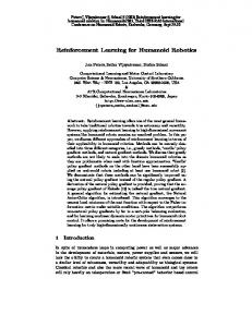
Current enterprise systems store petabytes of data on various storage devices (fast disks, slow disks, tapes) interconnected by storage area networks (SANs). As more data needs to be stored, new storage devices are connected to such networks. The currently available storage devices range widely in price and performance. For example, accessing a file on a new tape drive requires a robot to physically change the tape drives before the new data can be accessed, which can take several seconds (while data on disks can be accessed in milliseconds). For performance reasons, it is desirable to keep the most frequently accessed “hot” data on fast disks while keeping the old “cold” data on the inexpensive slow disks or tapes. Figure 1 shows an example of a multi-tier storage system. Unfortunately, the file access patterns change over time, and the data layout cannot be optimized once and for all. For example, in e-mail servers the file access frequency tends to decrease as files stay longer 2

Figure 1. Multi-tier Hierarchical Storage System.

in the system. The file access patterns in commercial Data Centers and Grids depend greatly on the clients connected to such systems at each point in time. Thus, online data migration has the potential to significantly increase performance of computing systems with hierarchical storage. Recently developed storage technologies (e.g., [8, 13]) allow transparent migration of files between storage tiers without affecting the running applications that are accessing them. However, the data migration policies they use are still based on some simple heuristics and no formal mathematical framework for minimizing the future I/O request response time has been developed. The Aqueduct system [6] uses a control-theoretic framework for dynamically adjusting the rate of background data migration to avoid Quality of Service (QoS) violations for the running applications. However, this system assumes that the data migration plan is given to it as an input. The STEPS architecture [19] for life cycle management in distributed file systems also uses feedback control to dynamically adjust the data migration rate. The migrations in that system are triggered by heuristic threshold-based policies such as IF space utilization in PREMIUM POOL is greater than 80%, THEN migrate .tmp files greater than 1MB ordered by size to IDLE POOL until the space utilization of PREMIUM POOL is 60%. A number of online data migration approaches have been proposed in the research community. However, the approaches we are aware of are reactive in nature: they suggest migrating “hot” files that have been accessed more frequently in the recent past to the faster storage tiers while swapping out the “coldest” files. As a representative example, [11] suggests estimating the expected cost of accessing each file based on the file location and on its estimated access frequency. A file is then upgraded to a faster tier of storage (e.g., from disk to a local cache) if the total cost of all files involved in this migration (such as those that need to be dropped from the cache) is reduced. The cost of accessing each file is dynamically estimated using a sliding average of accesses to similar objects in the recent past. While reactive approaches such as the one in [11] can definitely bring some benefit to multi-tier storage systems, they do not address several important system-level considerations. For example, reactive approaches do not consider the impact of migration overhead on the future response times of other files in the affected storage tiers, even though a constant migration overhead added to an overloaded storage tier can significantly increase its queuing delays. Therefore, the total benefit received by the transferred files needs to be weighed against the future impact of migration overhead in the particular states of the 3

affected storage tiers. The future response times of other files are also affected by changes in the file size distribution in each storage tier that result from file migrations. For example, the expected response times of all files in a storage tier will increase if a very large file is migrated into this tier, since the I/O requests to the original files will have to be queued for a long time while an I/O request for the very large file is served. Therefore, faster storage tiers have a preference for “hot” AND small files, and these two properties need to be traded off against each other on a case-by-case basis depending on the particular files and the states of the storage tiers involved in the migration. This paper presents a methodology for addressing the above tradeoffs by estimating the cost function for each storage tier – its expected future response time as a function of its current state. Given the cost functions for all storage tiers, the true impact of each migration decision can be easily estimated as the total change to the cost functions of the affected storage tiers that will result if the considered migration were to take place. This approach is consistent with the current industry trends of developing selfoptimizing systems, which make decisions that maximize a utility function rather than just following some built-in non-adaptive policies.

3

Hierarchical Storage System Model

Consider a multi-tier storage system as shown in Figure 1. Tier i has a limited bandwidth Bi , which is shared between file I/O requests and file transfers between the tiers (data migration). Multiple copies of a single file can be present in the storage system. Read/write/update requests arrive stochastically for each file. We assume that a certain policy already exists for routing new file write requests (a possible heuristic is to write the file to the fastest tier that has enough available space to fit this file). A file update request is routed to all tiers containing this file. A file read request is routed to the tier which has the smallest expected wait time out of the tiers containing this file. Requests at each tier form a queue and wait for their turn to be processed. The processing time for a read/write/update request for file k in tier i is the size of file k divided by Bi . File migrations can either be performed proactively or they can be triggered by I/O requests. The latter approach imposes a smaller load on the system, since the migration process in general contains the operation that would need to be executed while serving the I/O request (e.g., reading a file from some storage or writing a file to it). This consideration was found to be very important in our simulations of heavily loaded systems, since a small increase in the load (number of I/O operations that need to be executed) significantly increases the request response time in such systems. Therefore, the RL methodology will be applied in this paper to the I/O-triggered migration policies. When a file update request is received by some tier, the system decides whether this request should be routed instead to the next fastest tier, creating a new copy of the file in that tier and erasing the old copy present in the original tier. This consideration is made only if the file is not already present in the next fastest tier. When a file read request is received, the system first reads the file from disk and then decides whether this file should be upgraded to the next fastest tier. If an upgrade decision is made and not enough space is available in the faster tier, then some files are migrated out of that tier into the original tier. The migration-induced read/write operations are implemented as file requests that are sent to the corresponding tiers (that is, file migration operations do not take precedence over the regular file I/O requests). The decision to upgrade a file increases the queue length of the new tier and may also increase the queue length of the old tier if some large files need to be swapped out of the new tier. However, such a 4

decision may place the overall system into a more desirable state from the point of view of the expected future response time, if the file being upgraded is “hot” enough and the files being swapped out (if any) are “cold” enough. The objective is to design an automated policy for upgrading files so as to minimize the average system response time (possibly divided by the size of each request). The need for an automated migration policy extends to many different implementations of a multi-tier storage system, and some of the mechanisms described above can be easily modified without changing the spirit of the problem.

4

Solution Methodology

4.1

Defining and Using Cost Functions

This section addresses the first three issues (as was mentioned in the Introduction) that need to be resolved when applying RL to a real-world problem: deciding what intelligent agents the system will contain, choosing the variables to be used as inputs to the utility function of each agent, and deciding how the outputs of utility functions should be translated into actual data migration decisions. Since storage tiers generally possess different characteristics and can be dynamically added or removed from a multi-tier storage system, it is impractical to define a single utility function, mapping each possible data distribution among the tiers and properties of all the tiers into the expected future response time of I/O requests. Instead, we propose a scalable approach of viewing each storage tier as a separate decision-making entity (agent), allowing any pair of such agents to decide whether they want to redistribute the files among themselves at any point of time. In order to make data migration decisions, each storage tier (agent) learns its own long-term cost function C(s), which predicts the future average request response time divided by the file size (which will be called average weighted response time, AWRT), starting from a state s for the tier. An adequate state description is very important for learning such a function: the learning time for a given accuracy is exponential in the number of variables used to describe the state (so fewer variables are preferred), but at the same time all major influences on the future cost should be included so as to predict more accurately the future evolution of the agent’s state. Some methods are proposed in [7] for dynamically choosing the most appropriate set of features that an agent should use in making its decisions, trading off compactness vs. completeness. Such investigations, however, are outside of the scope of this work. The state vector s we used for each tier is based on the notion of “temperature” of each file, which approximates its access rate. In order to compute this estimate, the system keeps track of read/update requests for each file and uses these statistics to predict the probability of that file being accessed in the near future. More precisely, whenever a file k is accessed at time t, the system updates an estimate of the request interarrival time τk for this file: τk = ατk + (1 − α)(t − Lk ),

(1)

where Lk is the last access time for file k and α < 1 is a constant that determines how fast the past information should be discounted. The temperature Tk of file k is computed as Tk = 1/τk . The following state variables were then formed: • s1 = average temperature of all files stored and queued (those for which the write requests have already been received) in the tier. This variable predicts the number of accesses per unit of time 5

the tier will receive in the future. Note that if requests are infrequent and queuing does not occur, AWRT for each request to tier i is 1/Bi . Thus, a higher value of s1 suggests a higher probability of queuing and thus a larger expected cost C(s). • s2 = average weighted temperature of all files stored and queued in the tier (temperature multiplied by the file size). This variable predicts the amount of data that will be requested from the tier per unit of time in the future. For a given value of s1 , a higher value of s2 implies that larger files become relatively hotter, which suggests longer expected queuing times for requests to smaller files (many requests for small files need to wait for a long time while a single request for a large file is being processed) and hence a larger expected cost C(s). • s3 = current queuing time in the tier (wait time for a new request to start getting processed). This variable directly correlates with the queuing time for requests that arrive in the near future. The first two variables are likely to evolve gradually in real storage systems with many files per tier, and hence can be computed at regular time intervals that are large enough to allow for a noticeable change in these variables (e.g., a 1% change). Whenever a read/update request is received for file k that is not already in the fastest storage tier, the system decides whether this file should be upgraded to the next fastest tier, as described in Section 3. In order to make such a decision between tiers i and j, each of them computes its long term cost Cnot = C(state s if no migration is to take place) and Cup = C(state s˜ that would result after file k is upgraded). The file is then upgraded if j i j i Cup · s˜i1 + Cup · s˜j1 < Cnot · si1 + Cnot · sj1 ,

(2)

where si1 is the average temperature of all files in tier i if no migration is to take place and s˜i1 is the same quantity if the file in question were to be upgraded. The predicted average response time of a tier (cost) is multiplied by the tier temperature (s1 ) in the above migration criterion because AWRT for the multi-tier storage system can be computed as a weighted sum of AWRTs for all tiers, with the weights being the number of requests each tier has served, which is estimated by s1 . Note that once the tier cost functions C(s) are learned, any file reconfiguration decisions among the tiers can be evaluated using the criterion in equation (2). This approach is robust to tiers being added or removed from the system, is more scalable than centralized approaches and does not have a single point of failure inherent in centralized approaches. 4.2

Fuzzy Rulebase Representation of Cost Functions

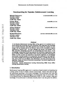
Any parameterized function approximation architecture can be used for representing the tier cost functions C(s) and then tuning them with RL. We will use a fuzzy rulebase (FRB) for this purpose because its structure and parameters can be easily interpreted, as will be explained below. An FRB is a function f that maps an input vector x ∈ 0 and ajn+1 = ajn /(1−ξnj δnj ) otherwise. As one can see, the above expressions imply a nonlinear tuning process for aj , for which no convergence guarantees have been developed so far. However, the experimental results presented in Section 6 demonstrate that additional tuning of these parameters leads to even better file migration policies.

11

4.6

A Different View of State Sampling During RL Updates

The standard closed-loop control environment (e.g., the RL problem formulation) assumes that effects of each action can only be observed at the next time step. Thus, the popular RL algorithms have focused on learning the optimal action a for each state s. In some real-world systems, however, the effect of each action can be immediately observed. This is often the case in systems that accept stochastically arriving jobs/requests and make some internal reconfigurations in response (e.g., storage environment considered in this paper, job scheduling environment [16], dynamic resource allocation [17]). In such cases, one can reduce the amount of noise present in RL updates by describing the system’s state in such a way so that effects of each action are reflected immediately in the system’s state. For example, whenever a decision is made to route a file request from one tier to another, all state variables listed in Section 4.1 are affected for both tiers and immediately reflect the new state of each tier. The particular RL methodology we propose for tuning the cost-to-go function parameters makes use of the above observation by specifying that the state sn in equation (8) is the one observed AFTER an upgrading decision (if any) is taken, while the state sn+1 is the one right BEFORE the next decision is made. That is, file migration decisions affect only the way the states are sampled for update in equation (8), but the evolution of a state sn to a state sn+1 is always governed by the fixed stochastic behavior of the multi-tier storage environment (which depends on the rates at which file requests are generated, file properties, tier properties, etc.). So far no theoretical convergence analysis has been performed for the proposed sampling approach of choosing at every decision point the smallest-cost state out of those that can be obtained (using the concept described in equation (7) and implemented in the migration criterion (2)), but our positive experimental results suggest its feasibility. Also note that the above view of the learning process as that of estimating the cost-to-go function for a fixed state transition policy eliminates the need for performing action exploration (which is necessary when we try to learn a new state transition policy), thus making it possible to use this approach online without degrading performance of the currently used policy. For example, if the cost-to-go function for some tier is initialized to prefer some obviously bad states, then after some period of learning the predicted costs of these states will rise to their real levels and the system will start avoiding those states when making scheduling decisions, without an explicit exploration having been performed. The simulation results in Section 6 demonstrate the power of the RL tuning approach by showing that very good policies can be learned even when the rule parameters pi are all initialized at 0 (no prior knowledge is used about the relative preferences of various system’s states) and the membership function parameters are initialized as described in Section 4.2.

5

Simulation Setup

The experimental results presented in Section 6 are based on a simulated two-tier storage system. Several simplifying assumptions were made about this storage system in order to make a more clear connection between the important system features and the relative performance of various file migration policies. We assumed 1000 files present in the system, with only one copy of each file being present. Each file stochastically changed its state between being “cold” and being “hot”. The probability of a cold file becoming hot after receiving an I/O request was 0.2 and the probability of a hot file becoming cold after receiving an I/O request was 0.005. Requests for a hot file were generated using a Poisson arrival process 12

with a rate of 0.5, and those for a cold file had an arrival rate of 0.01. The above numbers were chosen so as to result in approximately equal time periods of each file being hot and cold. That is, the average number of accesses a cold file stays cold is (1−ColdHotSwitchP rob)/ColdHotSwitchP rob = 4, and a hot file stays hot is (1 − HotColdSwitchP rob)/HotColdSwitchP rob = 199. The average number of time units a cold file stays cold is then 4/(ColdArrivalRate) = 400 and a hot file stays hot is 199/(HotArrivalRate) = 398. Read and write requests were equally probable for each file. At the start of every simulation, each file was initialized to be either hot or cold with probability 0.5. While real hierarchical storage systems will not have Poisson request arrival processes and 2-state Markov switching of files between being “cold” and “hot” (as assumed above), the above model is a reasonable approximation of the salient features of reality, according to domain experts we have consulted. Many researchers have observed that file sizes in the Internet data traffic have a Pareto distribution F (x) = 1 − (b/x)a for x ≥ b (e.g., [10]). We used this distribution with a = b = 1, since these values approximated well several practical workloads we had available. In order to decrease the variance of the experimental results, each simulation started with the same distribution of file sizes, resulting from a particular sampling of the assumed Pareto distribution. The following file sizes were sampled, in descending order of size: 1167, 655, 399, 271, 207, 175, 143, 128, 111, 95, 95. On the other side of the size spectrum, 500 files of size 1 were sampled from the Pareto distribution, 167 files of size 2 (up to file index 667), 83 files of size 3 (up to file index 750), 50 files of size 4 (up to file index 800), 33 files of size 4 (up to file index 833), etc. The storage capacity of the slow tier was chosen to be equal to the total size of all files in the system, 7511. The storage capacity of the fast tier was chosen to be 1/5 of that, 1502. The bandwidth of the slow tier was 1500, while that of the fast tier was 3000. The parameter updating rule in equation (8) is executed simultaneously for all tiers whenever each tier in the system has processed k or more requests since the last parameter update. If a very small value of k is used, each tier will not collect enough statistics about response times of requests served since the last update, and the learning will be very noisy. If a very large value of k is used, the parameter updates will be very infrequent, and the learning will be slow. We found experimentally that values between 5 and 50 resulted in statistically the same performance, which is shown in the next section. We have also experimented with different values for the discounting factor e−β used in equations (8) and (12), and found that values between 0.9 and 0.99 resulted in statistically the same optimal performance (presented in the next section), which then gradually degraded for values less than 0.9, since they made the RL algorithm more and more short-sighted. The total training period consisted of 20000 time steps, during which about 20000 parameter updates took place. The training period then followed by a testing period of 20000 time steps, during which the given file migration policy was evaluated. The final results (presented in Table 1) were averaged over 30 trials, making sure that the standard deviation of each performance number is less than 2% of the number itself. When determining the proper schedule for decreasing the learning rate αni in equation (8), we found that the standard approach of setting αni = 1/n decreased αni too fast, so that parameters pi werePnot able to reach their final values in 20000 time steps. However, when we used i αni = 0.1/(1 + N n−1 k=0 φ (sk )) with 50 < N < 500, the magnitudes of updates were large enough for i p to reach the neighborhood of their final values. The experimental results showed a slightly better performance when the learning rate ξnj used for updating the membership function parameters aj in equation (12) was kept constant rather than being decreased after every update. Note that the magnitude of δnj in equation (12) depends on the magnitude ˆ ∂C i of ∂a j , which in turn depends on the relative values of parameters p . Therefore, in order to have all 13

parameters aj updated at approximately the same constant rate, the expected value of ξnj δnj should be equal to the same small constant for all j. In order to achieve that, we first estimated for each j the average value δ¯nj of |δnj | during the first 5000 updates of parameters pi (while aj were not updated). We then found that setting ξnj = 0.001/δ¯nj resulted in reasonably sized updates. When using an FRB with membership functions µLj (xj ) = 1/(1+aj e−bj x ) and µSj (xj ) = 1−µLj (xj ) (as shown in Figure 2) to approximate some cost function, it is important to choose the initial values of parameters aj and bj appropriately. Assuming that aj are initially chosen so that µLj (xj ) and µSj (xj ) intersect at the mean value of xj , if bj is chosen too large, then µLj and µSj will look like step functions, while if bj is chosen too small, then µLj and µSj will look like two linear functions over the range of xj . As the practice shows, the maximal approximation capability of an FRB lies somewhere between the two extremes described above. In order to choose the appropriate value for bj , one has to first estimate the range of the values of xj . We achieve that by observing the storage system for the first 5000 time steps (making about 5000 file upgrading decisions) and computing the mean x¯j and the standard deviation σj for each variable xj . The expected range for xj (the one specified as [0,1] in Figure 2) is then set to be [¯ xj − 2 · σj , x¯j + 2 · σj ]. Let minXj = x¯j − 2 · σj , maxXj = x¯j + 2 · σj , Lj = maxXj − minXj , Cj = (maxXj + minXj )/2. We found that the value bj = 7.33/Lj as shown in Figure 2 resulted in the best approximations of the tier cost functions, which degraded gradually as bj was increased or decreased. The value of aj was then set to ebj Cj , so that µL (Cj ) = µS (Cj ) = 0.5. Note that given our choice for bj , all parameters aj were set to the same initial value of e0.5·7.33 . The parameters pi were all initialized to 0.

6

Simulation Results

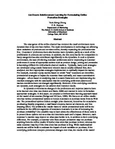
Table 1 shows the average weighted response time (AWRT) of the various policies considered. The first set of policies address the case when no file migration was performed and the policies differ only in the way the files were initially allocated in the system. In one case, each file, starting from the smallest one, was randomly assigned to one of the two tiers with equal probability if both tiers had enough space for it; otherwise, the file was written to the slow tier. In the other case, the smallest files were written to the fast tier until it became full (fitting 841 smallest files), at which point all remaining files were written to the slow tier. Note that AWRT for the second policy is 20 times smaller than that for the first policy! Such a large difference can be explained by the fact that it is very beneficial to keep all small files together and all large files together. Otherwise, small files can get stuck in the queue behind large files and experience a very large AWRT. All subsequent policies were initialized with the smallest-first allocation. The second set of results addresses the case of pre-specified file migration policies. In all of the cases file migration was found to give better results if files were upgraded only following a write request, which would simply be re-routed to the next fastest tier. That is, the slow tier most of the time did not experience any change in its load, since it would only have to execute the write requests for the files that were swapped out from the fast tier, which were together on average of the same size as the file being upgraded. However, when migration following a read request was enabled, the slow tier would actually experience an increase in its load, since it would have to first respond to the read request and then execute the write request for the files swapped out from the fast tier. The first two policies in this group address the case when a write request was routed from the slow tier to the fast tier if the file “temperature”, computed according to equation (1), was higher than that of 14

Policy

Cost (AWRT)

No Migration, random allocation

0.096

No Migration, smallest-first allocation

0.0043

Least Recently Used Replacement 1

0.085

Least Recently Used Replacement 2

0.027

Size-Temperature Replacement 1

0.0027

Size-Temperature Replacement 2

0.0026

RL Tuning of pi

0.0018

RL Tuning of pi and aj

0.0017

Table 1. Average Weighted Response Time (AWRT) of various policies

the “coldest” file in the fast tier. If the fast tier did not have enough space to accept the file, some files were swapped out to the slow tier, in the order of being least recently used (LRU). This file replacement policy is currently being used in most commercial storage products and also in managing CPU cache space. The first policy allowed all files to be upgraded, while the second policy allowed only files of size less than 200 to be upgraded. The second policy achieved a 3 time smaller AWRT because, once again, it prevented very large files from being in the same tier as most of the small files. However, it still allowed for a larger than desired mixing of large and small files, and consequently its AWRT was still 5 times larger than that of the no-migration policy with the smallest-first file allocation. Both of these policies (and all file migration policies discussed below) were given 5000 time steps at the beginning of the simulation to settle into a steady-state behavior, before the testing period (or the training period in the case of RL-based policies) began. The next two policies in this group used a replacement policy that considered both the temperature and the size of the files. This replacement policy would first try to remove a file that is of the same size or bigger and is also colder than the file being upgraded. If no such file was found, then the policy would try to remove at most two colder files that are of the same size or smaller, searching through all files in the order of decreasing size. If enough space could be created, the file was upgraded; otherwise, no action would be taken. That is, this replacement policy tried to simultaneously achieve the objectives of keeping hottest AND smallest files in the fast tier. The difference between these two policies is that the first one used the same upgrading criterion as before, while the second one used a stricter criterion of upgrading only those files that are hotter than the coldest file in the fast tier AND hotter than the average file temperature in the slow tier. As one can see, AWRT of these two policies is 10 times smaller than that of the policies based on LRU replacement. The final set of policies are those where migration was performed based on minimizing the tier cost functions, which were previously tuned with RL. More specifically, a write request would be forwarded to the fast tier if the migration criterion (2) was satisfied. The parameters were tuned using the TD(λ) RL algorithm presented in equations (8) and (12) using the whole range of possible values of λ. Interestingly, the difference in results between the various values of λ was statistically insignificant. Both policies allowed tuning the pi parameters, but only the second policy allowed a simultaneous tuning of the aj parameters as described in Section 5. We found that the values of parameters aj were changed by at most 15

50% regardless of the length of the training period. Recalling that parameters bj were set to 7.33/Lj , a 50% change in aj implies a shift of the intersection point between the membership functions µLj and µSj by about 5% of the range of the variable xj . A greater change was not observed possibly because the initial statistical estimate of this range (described in Section 5) was sufficiently accurate. That is, when statistical range estimation is used, the parameters aj do not really need to be tuned, and hence the results in Table 1 show only a minor performance improvement due to tuning aj . The parameter tuning process was based on a Policy Iteration (PI) approach, developed by Ronald Howard [3], which was previously mentioned when presenting equation (6). That is, during the first iteration the Size-Temperature Replacement 1 policy would be executed for 20000 time steps, and the tier cost functions Cj0 would be learned for this policy for tiers j = 1 and 2. During the second iteration, migration would be performed based on inequality (2) with the cost functions Cj0 , and the new cost functions Cj1 would be learned for this policy for 20000 time steps. During the third iteration, migration would be performed based on inequality (2) with the cost functions Cj1 , and the new cost functions Cj2 would be learned for this policy for 20000 time steps. It was found that statistically significant performance improvement was achieved only during the first three iterations of the PI cycle, reducing AWRT by 35% in comparison to the initial policy. This corresponds to the practical observations made by many researchers that the PI cycle can learn a very good policy after only several iterations. Another major practical benefit of the PI approach is that it never uses a “bad policy: each subsequent policy is at least as good as the previous one, making PI a good candidate for on-line learning. We are not aware of any successful attempts to tune the basis function parameters using RL, and some researchers in fact have reported that such a tuning decreases performance (e.g., [4, 15]). Therefore, the procedure presented in this paper for tuning aj is an important contribution to the practice of combining RL with function approximation architectures consisting of linear combinations of basis functions.

7

Conclusion

This paper presented a novel framework for dynamically re-distributing files in a multi-tier storage system, which explicitly minimizes the expected future average request response time. The previous approaches to storage system management are based on fixed heuristic policies and do not perform any performance optimization. The proposed framework uses a Reinforcement Learning (RL) methodology for tuning parameters of tier cost functions based on which file migration is performed. Any parameterized function approximation architecture can be used in the proposed framework to represent tier cost functions. A fuzzy rulebase architecture was chosen here for its ease of management. The RL methodology was applied to tuning the parameters of the fuzzy rulebase, which resulted in a 35% performance improvement relative to the best found pre-specified file migration policy. The experimental results were robust with respect to significant perturbations of the key parameters.

8

Acknowledgment

The author would like to thank Harriet Coverston from Sun Microsystems for the helpful information about hierarchical storage systems, as well as Declan Murphy and Victoria Livschitz for the help with presenting this material.

16

References [1] R. Das, G. J. Tesauro, W. E. Walsh. “Model-Based and Model-Free Approaches to Autonomic Resource Allocation,” IBM Technical Report RC23802, 2005. [2] S. W. Hasinoff. “Reinforcement Learning for Problems with Hidden State,” Technical Report, University of Toronto, Department of Computer Science, 2002. [3] R. A. Howard. Dynamic Programming and Markov Processes. John Wiley & Sons, Inc., New York, 1960. [4] R. M. Kretchmar and C. W. Anderson. “Comparison of CMACs and RBFs for Local Function Approximators in Reinforcement Learning.” In Proceedings of the IEEE International Conference on Machine Learning, pp. 834-837, Houston, TX, 1997. [5] L. J. Lin and T. M. Mitchell.“Memory Approaches to Reinforcement Learning in Non-Markovian Domain,” Carnegie Mellon School of Computer Science Technical Report CMU-CS-92-138, 1992. [6] C. Lu, G. A. Alvarez, and J. Wilkes. “Aqueduct: online data migration with performance guarantees,” Conference on File and Storage Technology (FAST’02), pp. 219 - 230, Monterey, CA, 2002. Published by USENIX, Berkeley, CA. [7] A. K. McCallum. Reinforcement Learning with Selective Perception and Hidden State, PhD. Thesis, University of Rochester, Department of Computer Science, 1995. [8] J. Menon, D. A. Pease, B. Rees, L. M. Duyanovich, and B. L. Hillsber. “IBM Storage Tank – A Heterogeneous Scalable SAN File System.” IBM Systems Journal, Vol. 42, No. 2, pp. 250 - 267, 2003. [9] N. Meuleau, L. Peshkin, K.-E. Kim, and L. P. Kaelbling. “Learning finite-state controllers for partially observable environments,” in Proceedings of the Fifteenth Conference on Uncertainty in Artificial Intelligence (UAI), pp. 427 – 436, 1999. [10] V. Paxson and S. Floyd. “Wide-Area Traffic: The Failure of Poisson Modeling.” IEEE/ACM Transactions on Networking, Vol. 3, No. 3, pp. 226 - 244, 1995. [11] M. Sinnwell and G. Weikum, “A Cost-Model-Based Online Method for Distributed Caching.” In Proceedings of the Thirteenth International Conference on Data Engineering (ICDE), pp. 532 - 541, Birmingham, UK, 1997. [12] R.S. Sutton and A. G. Barto. Reinforcement Learning: An Introduction. MIT Press, Cambridge, MA, 1998. [13] Sun Microsystems Inc. “Sun StorEdge QFS and SAM-FS Software,” Technical white paper. Available electronically at http://www.sun.com/storage/white-papers/qfs-samfs.pdf, 2004. [14] J. N. Tsitsiklis and B. Van Roy. “An Analysis of Temporal-Difference Learning with Function Approximation,” IEEE Transactions on Automatic Control, Vol. 42, No. 5, pp. 674 – 690, 1997. 17

[15] P. Vamplew and R. Ollington. “Global Versus Local Constructive Function Approximation for On-Line Reinforcement Learning.” Presented at the 18th Australian Joint Conference on Artificial Intelligence, December 5-9, Sydney, Australia, 2005. Published in Springer-Verlag Lecture Notes in Computer Science, Vol. 3809, pp. 113-121, 2005. [16] D. Vengerov. “Reinforcement Learning Framework for Utility-Based Scheduling in ResourceConstrained Systems.” Sun Microsystems Laboratories Technical Report TR-2005-141, Feb. 1, 2005. [17] D. Vengerov. “A Reinforcement Learning Approach to Dynamic Resource Allocation.” Sun Microsystems Laboratories Technical Report TR-2005-148, Sep. 1, 2005. [18] D. Vengerov. “Dynamic Tuning of Online Data Migration Policies in Hierarchical Storage Systems using Reinforcement Learning.” Sun Microsystems Laboratories Technical Report TR-2006-157, June 19, 2006. [19] A. Verma, U. Sharma, J. Rubas, D. Pease, M. Kaplan, R. Jain, M. Devarakonda and M. Beigi, “An Architecture for Lifecycle Management in Very Large File Systems,” In Proceedings of the 22nd IEEE / 13th NASA Goddard Conference on Mass Storage Systems and Technologies (MSST), pp. 160 - 168, 2005. [20] L.-X. Wang. “Fuzzy systems are universal approximators,” In Proceedings of the IEEE International Conference on Fuzzy Systems (FUZZ-IEEE ’92), pp. 1163 - 1169, 1992.

18