Data-Efficient Reinforcement Learning with Probabilistic Model ...

Data-Efficient Reinforcement Learning with Probabilistic Model Predictive Control

arXiv:1706.06491v2 [cs.SY] 22 Feb 2018

Sanket Kamthe Department of Computing Imperial College London

Abstract Trial-and-error based reinforcement learning (RL) has seen rapid advancements in recent times, especially with the advent of deep neural networks. However, the majority of autonomous RL algorithms require a large number of interactions with the environment. A large number of interactions may be impractical in many real-world applications, such as robotics, and many practical systems have to obey limitations in the form of state space or control constraints. To reduce the number of system interactions while simultaneously handling constraints, we propose a modelbased RL framework based on probabilistic Model Predictive Control (MPC). In particular, we propose to learn a probabilistic transition model using Gaussian Processes (GPs) to incorporate model uncertainty into longterm predictions, thereby, reducing the impact of model errors. We then use MPC to find a control sequence that minimises the expected long-term cost. We provide theoretical guarantees for first-order optimality in the GP-based transition models with deterministic approximate inference for long-term planning. We demonstrate that our approach does not only achieve state-of-the-art data efficiency, but also is a principled way for RL in constrained environments.

1

Introduction

Reinforcement learning (RL) is a principled mathematical framework for experience-based autonomous learnProceedings of the 21st International Conference on Artificial Intelligence and Statistics (AISTATS) 2018, Lanzarote, Spain. PMLR: Volume 84. Copyright 2018 by the author(s).

Marc Peter Deisenroth Department of Computing Imperial College London

ing of control policies. Its trial-and-error learning process is one of the most distinguishing features of RL [44]. Despite many recent advances in RL [25, 43, 48], a main limitation of current RL algorithms remains its data inefficiency, i.e., the required number of interactions with the environment is impractically high. For example, many RL approaches in problems with low-dimensional state spaces and fairly benign dynamics require thousands of trials to learn. This data inefficiency makes learning in real control/robotic systems without taskspecific priors impractical and prohibits RL approaches in more challenging scenarios. A promising way to increase the data efficiency of RL without inserting task-specific prior knowledge is to learn models of the underlying system dynamics. When a good model is available, it can be used as a faithful proxy for the real environment, i.e., good policies can be obtained from the model without additional interactions with the real system. However, modelling the underlying transition dynamics accurately is challenging and inevitably leads to model errors. To account for model errors, it has been proposed to use probabilistic models [42, 10]. By explicitly taking model uncertainty into account, the number of interactions with the real system can be substantially reduced. For example, in [10, 33, 1, 7], the authors use Gaussian processes (GPs) to model the dynamics of the underlying system. The PILCO algorithm [10] propagates uncertainty through time for long-term planning and learns parameters of a feedback policy by means of gradient-based policy search. It achieves an unprecedented data efficiency for learning control policies for from scratch. While the PILCO algorithm is data efficient, it has few shortcomings: 1) Learning closed-loop feedback policies needs the full planning horizon to stabilise the system, which results in a significant computational burden; 2) It requires us to specify a parametrised policy a priori, often with hundreds of parameters; 3) It cannot handle state constraints; 4) Control constraints are enforced by using a differentiable squashing function that is applied

Sanket Kamthe, Marc Peter Deisenroth

to the RBF policy. This allows PILCO to explicitly take control constraints into account during planning. However, this kind of constraint handling can produce unreliable predictions near constraint boundaries [41, 26, 22]. In this paper, we develop an RL algorithm that is a) data efficient, b) does not require to look at the full planning horizon, c) handles constraints naturally, d) does not require a parametrised policy, e) is theoretically justified. The key idea is to reformulate the optimal control problem with learned GP models as an equivalent deterministic problem, an idea similar to [27]. This reformulation allows us to exploit Pontryagin’s maximum principle to find optimal control signals while handling constraints in a principled way. We propose probabilistic model predictive control (MPC) with learned GP models, while propagating uncertainty through time. The MPC formulation allows to plan ahead for relatively short horizons, which limits the computational burden and allows for infinite-horizon control applications. Our approach can find optimal trajectories in constrained settings, offers an increased robustness to model errors and an unprecedented data efficiency compared to the state of the art.

tions [5, 33]. The AICO model [47] uses approximate inference with (known) locally linear models. The probabilistic trajectories for model-free RL in [40] are obtained by reformulating the stochastic optimal control problem as KL divergence minimisation. We implicitly linearise the transition dynamic via moment matching approximation. Contribution The contributions of this paper are the following: 1) We propose a new ‘deterministic’ formulation for probabilistic MPC with learned GP models and uncertainty propagation for long-term planning. 2) This reformulation allows us to apply Pontryagin’s Maximum Principle (PMP) for the open-loop planning stage of probabilistic MPC with GPs. Using the PMP we can handle control constraints in a principled fashion while still maintaining necessary conditions for optimality. 3) The proposed algorithm is not only theoretically justified by optimal control theory, but also achieves a state-of-the-art data efficiency in RL while maintaining the probabilistic formulation. 4) Our method can handle state and control constraints while preserving its data efficiency and optimality properties.

2 Related Work Model-based RL: A recent survey of model based RL in robotics [35] highlights the importance of models for building adaptable robots. Instead of GP dynamics model with a zero prior mean (as used in this paper) an RBF network and linear mean functions are proposed [7, 3]. This accelerates learning and facilitates transferring a learned model from simulation to a real robot. Even implicit model learning can be beneficial: The UNREAL learner proposed in [17] learns a predictive model for the environment as an auxiliary task, which helps learning. MPC with GP transition models: GP-based predictive control was used for boiler and building control [13, 28], but the model uncertainty was discarded. In [18], the predictive variances were used within a GP-MPC scheme to actively reject periodic disturbances, although not in an RL setting. Similarly, in [31, 32], the authors used a GP prior to model additive noise and model is improved episodically. In [5, 28], the authors considered MPC problems with GP models, where only the GP’s posterior mean was used while ignoring the variance for planning. MPC methods with deterministic models are useful only when model errors and system noise can be neglected in the problem [19, 12]. Optimal Control: The application of optimal control theory for the models based on GP dynamics employs some structure in the transition model, i.e., there is an explicit assumption of control affinity [16, 33, 34, 5] and linearisation via locally quadratic approxima-

Controller Learning via Probabilistic MPC

We consider a stochastic dynamical system with states x ∈ RD and admissible controls (actions) u ∈ U ⊂ RU , where the state follows Markovian dynamics xt+1 = f (xt , ut ) + w

(1)

with an (unknown) transition function f and i.i.d. sys2 tem noise w ∼ N (0, Q), where Q = diag(σ12 , . . . , σD ). In this paper, we consider an RL setting where we seek control signals u∗0 , . . . , u∗T −1 that minimise the expected long-term cost J = E[Φ(xT )] +

XT −1 t=0

E[`(xt , ut )] ,

(2)

where Φ(xT ) is a terminal cost and `(xt , ut ) the stage cost associated with applying control ut in state xt . We assume that the initial state is Gaussian distributed, i.e., p(x0 ) = N (µ0 , Σ0 ). For data efficiency, we follow a model-based RL strategy, i.e., we learn a model of the unknown transition function f , which we then use to find open-loop1 optimal controls u∗0 , . . . , u∗T −1 that minimise (2). After every application of the control sequence, we update the learned model with the newly acquired experience 1

‘Open-loop’ refers to the fact that the control signals are independent of the state, i.e., there is no state feedback incorporated.

Sanket Kamthe, Marc Peter Deisenroth

and re-plan. Section 2.1 summarises the model learning step; Section 2.2 details how to obtain the desired open-loop trajectory. 2.1

Probabilistic Transition Model

We learn a probabilistic model of the unknown underlying dynamics f to be robust to model errors [42, 10]. In particular, we use a Gaussian process (GP) as a prior p(f ) over plausible transition functions f . A GP is a probabilistic non-parametric model for regression. In a GP, any finite number of function values is jointly Gaussian distributed [39]. A GP is fully specified by a mean function m(·) and a covariance function (kernel) k(·, ·). The inputs for the dynamics GP are given by tuples et := (xt , ut ), and the corresponding targets are xt+1 . x We denote the collections of training inputs and targets f y, respectively. Furthermore, we assume a Gausby X, sian (RBF, squared exponential) covariance function
ej ) = σf2 exp − 12 (e ej )T L−1 (e ej ) , (3) k(e xi , x xi − x xi − x where σf2 is the signal variance and L = diag(l1 , . . . , lD+U ) is a diagonal matrix of length-scales l1 , . . . , lD+U . The GP is trained via the standard procedure of evidence maximisation [21, 39]. We make the standard assumption that the GPs for each target dimension of the transition function f : RD × U → RD are independent. For given hyperf training targets y and a parameters, training inputs X, e∗ , the GP yields the predictive distribunew test input x f y) = N (f (e tion p(f (e x∗ )|X, x∗ )|m(e x∗ ), Σ(e x∗ )), where m(e x∗ ) = [m1 (e x∗ ), . . . , mD (e x∗ )]T

(4)

2 −1 f md (e x∗ ) = kd (e x∗ , X)(K yd d + σd I)
2 Σ(e x∗ ) = diag σ12 (e x∗ ), . . . , σD (e x∗ )

(5)

σd2

=

σf2d

(6)

2 −1 f fx e∗ ) , (7) − kd (e x∗ , X)(K kd (X, d + σd I)

for all predictive dimensions d = 1, . . . , D. 2.2

Open-Loop Control

To find the desired open-loop control sequence u∗0 , . . . , u∗T −1 , we follow a two-step procedure proposed in [10]. 1) Use the learned GP model to predict the long-term evolution p(x1 ), . . . , p(xT ) of the state for a given control sequence u0 , . . . , uT −1 . 2) Compute the corresponding expected long-term cost (2) and find an open-loop control sequence u∗0 , . . . , u∗T −1 that minimises the expected long-term cost. In the following, we will detail these steps.

2.2.1

Long-term Predictions

To obtain the state distributions p(x1 ), . . . , p(xT ) for a given control sequence u0 , . . . , uT −1 , we iteratively predict ZZ p(xt+1 |ut ) = p(xt+1 |xt , ut )p(xt )p(f )df dxt (8) for t = 0, . . . , T − 1 , by making a deterministic Gaussian approximation to p(xt+1 |ut ) using moment matching [12, 37, 10]. This approximation has been shown to work well in practice in RL contexts [10, 1, 7, 2, 3, 33, 34] and can be computed in closed form when using the Gaussian kernel (3). A key property that we exploit is that moment matching allows us to formulate the uncertainty propagation in (8) as a ‘deterministic system function’ zt+1 = fM M (zt , ut ) ,

zt := [µt , Σt ] ,

(9)

where µt , Σt are the mean and the covariance of p(xt ). For a deterministic control signal ut we further define the moments of the control-augmented distribution p(xt , ut ) as e t ], µ e t = blkdiag[Σt , 0] , (10) et, Σ e t = [µt , ut ], Σ zet := [µ such that (9) can equivalently be written as the deterministic system equation zt+1 = fM M (e zt ) . 2.2.2

(11)

Optimal Open-Loop Control Sequence

To find the optimal open-loop sequence u∗0 , . . . , u∗T −1 , we first compute the expected long-term cost J in (2) using the Gaussian approximations p(x1 ), . . . , p(xT ) obtained via (8) for a given open-loop control sequence u0 , . . . , uT −1 . Second, we find a control sequence that minimises the expected long-term cost (2). In the following, we detail these steps. Computing the Expected Long-Term Cost To compute the expected long-term cost in (2), we sum up the expected immediate costs Z e t )de et, Σ E[`(xt , ut )] = `(e xt )N (e xt |µ xt (12) for t = 0, . . . , T − 1. We choose `, such that this expectation and the partial derivatives ∂E[`(xt , ut )]/∂xt , ∂E[`(xt , ut )]/∂ut can be computed analytically.2 2 Choices for ` include the standard quadratic (polynomial) cost, but also costs expressed as Fourier series expansions or radial basis function networks with Gaussian basis function.

Sanket Kamthe, Marc Peter Deisenroth

Similar to (9), this allows us to define deterministic mappings `M M (zt , ut ) = `M M (e zt ) := E[`(xt , ut )]

(13)

ΦM M (zT ) := E[Φ(xT )]

(14)

e onto the correthat map the mean and covariance of x sponding expected costs in (2). Remark 1. The open-loop optimisation turns out to be sparse [4]. However, optimisation via the value function or dynamic programming is valid only for unconstrained controls. To address this practical shortcoming, we define Pontryagin’s Maximum Principle that allows us to formulate the constrained problem while maintaining the sparsity. We detail this sparse structure for the constrained GP dynamics problem in section 3. 2.3

Feedback Control with MPC

Thus far, we presented a way for efficiently determining an open-loop controller. However, an open-loop controller cannot stabilise the system [22]. Therefore, it is essential to obtain a feedback controller. MPC is a practical framework for this [22, 15]. While interacting with the system MPC determines an H-step open-loop control trajectory u∗0 , . . . , u∗H−1 , starting from the current state xt 3 . Only the first control signal u∗0 is applied to the system. When the system transitions to xt+1 , we update the GP model with the newly available information, and MPC re-plans u∗0 , . . . , u∗H−1 . This procedure turns an open-loop controller into an implicit closedloop (feedback) controller by repeated re-planning H steps ahead from the current state. Typically, H  T , and MPC even allows for T = ∞. In this section, we provided an algorithmic framework for probabilistic MPC with learned GP models for the underlying system dynamics, where we explicitly use the GP’s uncertainty for long-term predictions (8). In the following section, we will justify this using optimal control theory. Additionally, we will discuss how to account for constrained control signals in a principled way without the necessity to warp/squash control signals as in [10].

3

only depend on variables with neighbouring time index, i.e., ∂J/∂ut depends only variables with index t and t + 1. Furthermore, it allows us to explicitly deal with constraints on states and controls. In the following, we detail how to solve the optimal control problem (OCP) with PMP for learned GP dynamics and deterministic uncertainty propagation. We additionally provide a computationally efficient way to compute derivatives based on the maximum principle. To facilitate our discussion we first define some notation. Practical control signals are often constrained. We formally define a class of admissible controls U that are piecewise continuous functions defined on a compact space U ⊂ RU . This definition is fairly general, and commonly used zero-order-hold or first-order-hold signals satisfy this requirement. Applying admissible controls to the deterministic system dynamics fM M defined in (11) yields a set Z of admissible controlled trajectories. We define the tuple (Z, fM M , U) as our control system. For a single admissible control trajectory u0:H−1 , there will be a unique trajectory z0:H , and the pair (z0:H , u0:H−1 ) is called an admissible controlled trajectory [41]. We now define the control-Hamiltonian [6, 41, 45] for this control system as H(λt+1 , zt , ut ) = `M M (zt , ut ) + λTt+1 fM M (zt , ut ). (15) This formulation of the control-Hamiltonian is the centre piece of the Pontryagin’s approach to the OCP. The vector λt+1 can be viewed as a Lagrange multiplier for dynamics constraints associated with the OCP [6, 41]. To successfully apply PMP we need the system dynamics to have a unique solution for a given control sequence. Traditionally, this is interpreted as the system is ‘deterministic’. This interpretation has been considered a limitation of PMP [45]. In this paper, however, we exploit the fact that the moment-matching approximation (8) is a deterministic operator, similar to the projection used in EP [30, 23]. This yields the ‘deterministic’ system equations (9), (11) that map moments of the state distribution at time t to moments of the state distribution at time t + 1.

Theoretical Justification 3.1

Bellman’s optimality principle [1] yields a recursive formulation for calculating the total expected cost (2) and gives a sufficient optimality condition. PMP [36] provides the corresponding necessary optimality condition. PMP allows us to compute gradients ∂J/∂ut of the expected long-term cost w.r.t. the variables that 3

A state distribution p(xt ) would work equivalently in our framework.

Existence/Uniqueness of a Local Solution

To apply the PMP we need to extend some of the important characteristics of ODEs to our system. In particular, we need to show the existence and uniqueness of a (local) solution to our difference equation (11). For existence of a solution we need to satisfy the difference equation point-wise over the entire horizon and for uniqueness we need the system to have only one

Sanket Kamthe, Marc Peter Deisenroth

singularity. For our discrete-time system equation (via the moment-matching approximation) in (9) we have the following Lemma 1. The moment matching mapping fM M is Lipschitz continuous for controls defined over a compact set U. The proof is based on bounding the gradient of fM M and detailed in the supplementary material. Existence and uniqueness of the trajectories for the moment matching difference equation are given by Lemma 2. A solution of zt+1 = fM M (zt , ut ) exists and is unique. Proof Sketch Difference equations always yield an answer for a given input. Therefore, a solution trivially exists. Uniqueness directly follows from the PicardLindelöf theorem, which we can apply due to Lemma 1. This theorem requires the discrete-time system function to be deterministic (see Appendix B of [41]). Due to our re-formulation of the system dynamics (9), this follows directly, such that the z1:T for a given control sequence u0:T −1 are unique. 3.2

Pontryagin’s Maximum Principle for GP Dynamics

With Lemmas 1 2 and the definition of the controlHamiltonian 15 we can now state PMP for the control system (Z, fM M , U) as follows: Theorem 1. Let (zt∗ , u∗t ), 0 ≤ t ≤ H − 1 be an admissible controlled trajectory defined over the horizon ∗ H. If (z0:H , u∗0:H−1 ) is optimal, then there exists an ad-joint vector λt ∈ RD \ {0} satisfying the following conditions: 1. Ad-joint equation: The ad-joint vector λt is a solution to the discrete difference equation λTt =

∂ ∂fM M (zt , ut ) `M M (zt , ut ) + λTt+1 . ∂zt ∂zt

(16)

2. Transversality condition: At the endpoint the adjoint vector λH satisfies λH =

∂ ΦM M (zH ) . ∂zH

(17)

3. Minimum Condition: For t = 0, . . . , H − 1, we have

For every t = 0, . . . , H − 1 we find optimal controls u∗t ∈ arg minν H(λt+1 , zt∗ , ν). The minimisation problem possesses additional variables λt+1 . These variables can be interpreted as Lagrange multipliers for the optimisation. They capture the impact of the control ut over the whole trajectory and, hence, these variables make the optimisation problem sparse [11]. For the GP dynamics we compute the multipliers λt in closed form, thereby, significantly reducing the computational burden to minimise the expected long-term cost J in (2). We detail this calculation in section 3.3. Remark 3. In the optimal control problem, we aim to find an admissible control trajectory that minimizes the cost subject to possibly additional constraints. PMP gives first-order optimality conditions over these admissible controlled trajectories and can be generalised to handle additional state and control constraints [45, 26, 41]. Remark 4. The Hamiltonian H in (18) is constant for unconstrained controls in time-invariant dynamics and equals 0 everywhere when the final time H is not fixed [41]. Remark 5. For linear dynamics the proposed method is a generalisation of iLQG [46]: The moment matching transition fM M implicitly linearises the transition dynamics at each time step, whereas in iLQG an explicit local linear approximation is made. For a linear fM M and a quadratic cost ` we can write the LQG case as shown in Theorem 1 in [47]. If we iterate with successive corrections to the linear approximations we obtain iLQG. 3.3

Efficient Gradient Computation

With the definition of the Hamiltonian H in (15) we can efficiently calculate the gradient of the expected total cost J. For a time horizon H we can write the accumulated cost as the Bellman recursion [1] JH (zH ) := ΦM M (zH ), Jt (zt ) := `M M (zt , ut ) + Jt+1 (zt+1 )

(19) (20)

for t = H − 1, . . . , 0. Since the (open-loop) control ut only impacts the future costs via zt+1 = fM M (zt , ut ) the derivative of the total cost with ut is given by ∂Jt ∂`M M (zt , ut ) ∂Jt+1 ∂fM M (zt , ut ) = + . (21) ∂ut ∂ut ∂zt+1 ∂ut

(18)

Comparing this expression with the definition of the Hamiltonian (15), we see that if we make the substitu∂Jt+1 tion λTt+1 = ∂z we obtain t+1

Remark 2. The minimum condition (18) can be used to find an optimal control. The Hamiltonian is minimised point-wise over the admissible control set U:

∂Jt ∂`M M (zt , ut ) ∂fM M (zt , ut ) H = + λTt+1 = . ∂ut ∂ut ∂ut ∂ut (22)

H(λt+1 , zt∗ , u∗t ) = min H(λt+1 , zt∗ , ν) ν

for all ν ∈ U.

Sanket Kamthe, Marc Peter Deisenroth

This implies that the gradient of the expected longterm cost w.r.t. ut can be efficiently computed using the Hamiltonian [45]. Next we show that the substi∂Jt+1 tution λTt+1 = ∂z is valid for the entire horizon H. t+1 For the terminal cost ΦM M (zH ) this is valid by the transversality condition (17). For other time steps we differentiate (19) w.r.t. zt , which yields ∂`M M (zt , ut ) ∂Jt+1 ∂zt+1 ∂Jt = + ∂zt ∂zt ∂zt+1 ∂zt ∂`M M (zt , ut ) ∂fM M (zt , ut ) = + λTt+1 , ∂zt ∂zt

(23) (24)

which is identical to the ad-joint equation (16). Hence, in our setting, PMP implies that gradient descent on the Hamiltonian H is equivalent to gradient descent on the total cost (2) [41, 11]. Algorithmically, in an RL setting, we find the optimal control sequence u∗0 , . . . , u∗H−1 as follows: 1. For a given initial (random) control sequence u0:H−1 we follow the steps described in section 2.2.1 to determine the corresponding trajectory z1:H . Addition∂Jt+1 ally, we compute Lagrange multipliers λTt+1 = ∂z t+1 during the forward propagation. Note that traditionally ad-joint equations are propagated backward to find the multipliers [6, 41]. 2. Given λt and a cost function `M M we can determine the Hamiltonians H1:H . Then we find a new control sequence u∗0:H−1 via any gradient descent method using (22). 3. Return to 1 or exit when converged. We use Sequential Quadratic Programming (SQP) with BFGS for Hessian updates [29]. The Lagrangian of SQP is a partially separable function [14]. In the PMP, this separation is explicit via the Hamiltonians, i.e., the Ht is a function of variables with index t or t+1. This leads to a block-diagonal Hessian of SQP Lagrangian [14]. The structure can be exploited to approximate the Hessian via block-updates within BFGS [14, 4]

4

Experimental Results

We evaluate the quality of our algorithm in two ways: First, we assess whether probabilistic MPC leads to faster learning compared with PILCO, the current state of the art in terms of data efficiency. Second, we assess the impact of state constraints while performing the same task. We consider two RL benchmark problems: the underactuated cart-pole-swing-up and the fully actuated double-pendulum swing-up. In both tasks, PILCO is the most data-efficient RL algorithm to date [1].

u1

u u2 (a) Cart-pole with constraint.

(b) Double pendulum with constraint.

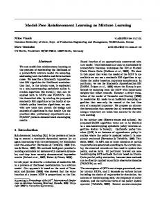
Figure 1: State constraints in RL benchmarks. (a) The position of the cart is constrained on the left side by a wall. (b) The angle of the inner pendulum cannot enter the grey region.

Under-actuated Cart-Pole Swing-Up The cart pole system is an under-actuated system with a freely swinging pendulum of 50 cm mounted on a cart. The swing-up and balancing task cannot be solved using a linear model [38]. The cart-pole system state space consists of the position of the cart x, cart velocity x, ˙ ˙ the angle θ of the pendulum and the angular velocity θ. A horizontal force u ∈ [−10, 10] N can be applied to the cart. Starting in a position where the pendulum hangs downwards, the objective is to automatically learn a controller that swings the pendulum up and balances it in the inverted position in the middle of the track. Constrained Cart-Pole Swing-Up For the statespace constraint experiment we place a wall on the track near the target, see Fig. 1(a). The wall is at -70 cm, which, along with force limitations, requires the system to swing from the right side. Fully-actuated Double-Pendulum The double pendulum system is a two-link robot arm (links lengths: 1 m) with two actuators at each joint. The state space consists of 2 angles and 2 angular velocities [θ1 , θ2 , θ˙1 , θ˙2 ] [1]. The torques u1 and u2 are limited to [−2, 2] Nm. Starting from a position where both links are in a downwards position, the objective is to learn a control strategy that swings the double-pendulum up and balances it in the inverted position. Constrained Double-Pendulum The doublependulum has a constraint on the angle of the inner pendulum, so that it only has a 340◦ motion range, i.e., it cannot spin through, see Fig. 1(b). The constraint blocks all clockwise swing-ups. The system is underpowered, and it has to swing clockwise first for a counter-clockwise swing-up without violating the constraints.

Baselines We compare our GP-MPC approach with the following baselines: the PILCO algorithm [10, 1] and a zero-variance GP-MPC algorithm (in the flavour of [28, 5]) for RL, where the GP’s predictive variances are discarded. Due to the lack of exploration, such a zero-variance approach within PILCO (a policy search method) does not learn anything useful as already demonstrated in [1], and we do not include this baseline. We average over 10 independent experiments, where every algorithm is initialised with the same first (random) trajectory. The performance differences of the RL algorithms are therefore due to different approaches to controller learning and the induced exploration. 4.1

Data Efficiency

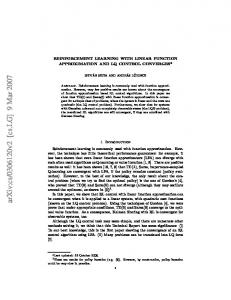
In both benchmark experiments (cart-pole and double pendulum), we use the exact saturating cost from [1], which penalises the Euclidean distance of the tip of the (outer) pendulum from the target position, i.e., we are in a setting in which PILCO performs very well. Fig. 2(a) shows that both our MPC-based controller (blue) and the zero-variance approach successfully4 complete the task in fewer trials than the state-of-theart PILCO method (red). From the repeated trials we see that GP-MPC learns faster and more reliably than PILCO. In particular, GP-MPC and the zerovariance approach can solve the cart-pole task with high probability (90%) after three trials (9 seconds), where the first trial was random. PILCO needs two additional trials. The reason why the zero-variance approach (no model uncertainties) works in an MPC context but not within a policy search setting is that we include every observed state transition immediately in the GP dynamics model, which makes MPC fairly robust to model errors. It even allows for model-based RL with deterministic models in simple settings. Fig. 2(b) highlights that our proposed GP-MPC approach (yellow) requires on average only six trials (18 s) 4 We define ‘success’ if the pendulum tip is closer than 8 cm to the target position for ten consecutive time steps.

PILCO GP-MPC Zero-Var

Trial # (3 sec per trial)

(a) Under-actuated cart-pole swing-up.

Success %

Trials The general setting is as follows: All RL algorithms start off with a single short random trajectory, which is used for learning the dynamics model. As in [10, 1] the GP is used to predict state differences xt+1 − xt . The learned GP dynamics model is then used to determine a controller based on iterated moment matching (8), which is then applied to the system, starting from x0 ∼ p(x0 ). Model learning, controller learning and application of the controller to the system constitute a ‘trial’. After each trial, the hyper-parameters of the model are updated with the newly acquired experience and learning continues.

Success %

Sanket Kamthe, Marc Peter Deisenroth

PILCO GP-MPC Zero-Var

Trial # (3 sec per trial)

(b) Fully-actuated double-pendulum swing-up.

Figure 2: Performance of RL algorithms. Error bars represent the standard error. (a) Cart-pole; (b) Double pendulum. GP-MPC (blue) consistently outperforms PILCO (red) and the zero-variance MPC approach (yellow) in terms of data efficiency. While the zero-variance MPC approach works well on the cart-pole task, it fails in the double-pendulum task. We attribute this to the inability to explore the state space sufficiently well. of experience to achieve a 90% success rate5 , including the first random trial. PILCO requires four additional trials, whereas the zero-variance MPC approach completely fails in this RL setting. The reason for this failure is that the deterministic predictions with a poor model in this complicated state space do not allow for sufficient exploration. We also observe that GP-MPC is more robust to the variations amongst trials. In both experiments, our proposed GP-MPC requires only 60% of PILCO’s experience, such that we report an unprecedented learning speed for these benchmarks, even with settings for which PILCO performs very well. We identify two key ingredients that are responsible for the success and learning speed of our approach: the ability to (1) immediately react to observed states by adjusting the long-term plan and (2) augment the training set of the GP model on the fly as soon as a new state transition is observed (hyper-parameters are not updated at every time step). These properties turn out to be crucial in the very early stages of learning 5 The tip of outer pendulum is closer than 22 cm to the target.

Sanket Kamthe, Marc Peter Deisenroth

Success %

Experiment PILCO GP-MPC-Mean GP-MPC-Var PILCO GP-MPC-Var GP-MPC-Mean

Cart-pole 16/100 21/100 3/100

Double Pendulum 23/100 26/100 11/100

Table 1: State constraint violations. The number of trials that resulted in state constraint violation corresponding to the trial data shown in the the Fig. 3.

Trial # (3 sec or less per trial)

(a) Cart-pole with constraint.

Success %

PILCO GP-MPC-Var GP-MPC-Mean

Trial # (3 sec or less per trial)

(b) Double pendulum with constraint.

Figure 3: Performance with state-space constraints. Error bars represent the standard error. (a) Cart-pole; (b) Double pendulum.GP-MPC with chance constraints. GP-MPC-Var (blue) is the only method that is able to consistently solve the problem. Expected violations constraint GP-MPC-Mean (yellow) fails in cart-pole. PILCO (red) violates state constraints and struggles to complete the task.

when very little information is available. If we ignored the on-the-fly updates of the GP dynamics model, our approach would still successfully learn, although the learning efficiency would be slightly decreased. 4.2

State Constraints

A scenario in which PILCO struggles is a setting with state space constraints. We modify the cart-pole and the double-pendulum tasks to such a setting. Both tasks are symmetric, and we impose state constraints in such a way that only one direction of the swing-up is feasible. For the cart-pole system, we place a wall near the target position of the cart, see Fig. 1(a); the double pendulum has a constraint on the angle of the inner pendulum, so that it only has a 340◦ motion range, i.e., it cannot spin through, see Fig. 1(b). These constraints constitute linear constraints on the state. We use a quadratic cost that penalises the Euclidean distance between the tip of the pendulum and the target. This, along with the ‘implicit’ linearisation, makes the optimal control problem an ‘implicit’ QP. If a rollout violates the state constraint we immediately

abort that trial and move on to the next trial. We use the same experimental set-up as data efficiency experiments. The state constraints are implemented as expected violations, i.e., E[xt ] < xlimit and chance constraints p(xt < xlimit ) ≥ 0.95. Fig. 1(a) shows that our MPCbased controller with chance constraint (blue) successfully completes the task with a small acceptable number of violations, see Table 1. The expected violation approach, which only considers the predicted mean (yellow) fails to complete the task due to repeated constraint violations. PILCO uses its saturating cost (there is little hope for learning with quadratic cost [8]) and has partial success in completing the task, but it struggles, especially during initial trials due to repeated state violations. One of the key points we observe from the Table 1 is that the incorporation of uncertainty into planning is again crucial for successful learning. If we use only predicted means to determine whether the constraint is violated, learning is not reliably ‘safe’. Incorporation of the predictive variance, however, results in significantly fewer constraint violations.

5

Conclusion and Discussion

We proposed an algorithm for data-efficient RL that is based on probabilistic MPC with learned transition models using Gaussian processes. By exploiting Pontryagin’s maximum principle our algorithm can naturally deal with state and control constraints. Key to this theoretical underpinning of a practical algorithm was the re-formulation of the optimal control problem with uncertainty propagation via moment matching into an deterministic optimal control problem. MPC allows the learned model to be updated immediately, which leads to an increased robustness with respect to model inaccuracies. We provided empirical evidence that our framework is not only theoretically sound, but also extremely data efficient, while being able to learn in settings with hard state constraints. One of the most critical components of our approach is the incorporation of model uncertainty into modelling and planning. In complex environments, model

Sanket Kamthe, Marc Peter Deisenroth

uncertainty drives targeted exploration. It additionally allows us to account for constraints in a risk-averse way, which is important in the early stages of learning.

References [1] R. E. Bellman. Dynamic Programming. Princeton University Press, Princeton, NJ, USA, 1957. [2] B. Bischoff, D. Nguyen-Tuong, T. Koller, H. Markert, and A. Knoll. Learning Throttle Valve Control Using Policy Search. In Proceedings of the European Conference on Machine Learning and Knowledge Discovery in Databases, 2013. [3] B. Bischoff, D. Nguyen-Tuong, H. van Hoof, A. McHutchon, C. E. Rasmussen, A. Knoll, J. Peters, and M. P. Deisenroth. Policy Search for Learning Robot Control using Sparse Data. In Proceedings of the International Conference on Robotics and Automation, 2014. [4] H. G. Bock and K. J. Plitt. A Multiple Shooting Algorithm for Direct Solution of Optimal Control Problems. In Proceedings 9th IFAC World Congress Budapest. Pergamon Press, 1984. [5] J. Boedecker, J. T. Springenberg, J. Wulfing, and M. Riedmiller. Approximate Real-time Optimal Control based on Sparse Gaussian Process Models. In Symposium on Adaptive Dynamic Programming and Reinforcement Learning, 2014. [6] F. H. Clarke. Optimization and Non-Smooth Analysis. Society for Industrial and Applied Mathematics, 1990. [7] M. Cutler and J. P. How. Efficient Reinforcement Learning for Robots using Informative Simulated Priors. In Proceedings of the International Conference on Robotics and Automation, 2015. [8] M. P. Deisenroth Efficient Reinforcement Learning using Gaussian Processes. KIT Scientific Publishing, 2010. [9] M. P. Deisenroth, D. Fox, and C. E. Rasmussen. Gaussian Processes for Data-Efficient Learning in Robotics and Control. Transactions on Pattern Analysis and Machine Intelligence, 37(2):408–23, 2015. [10] M. P. Deisenroth and C. E. Rasmussen. PILCO: A Model-Based and Data-Efficient Approach to Policy Search. In Proceedings of the International Conference on Machine Learning, 2011. [11] M. Diehl. Lecture Notes on Optimal Control and Estimation. 2014. [12] A. Girard, C. E. Rasmussen, J. QuinoneroCandela, and R. Murray-Smith. Gaussian Process Priors with Uncertain Inputs-Application to

Multiple-Step Ahead Time Series Forecasting. Advances in Neural Information Processing Systems, 2003. [13] A. Grancharova, J. Kocijan, and T. A. Johansen. Explicit Stochastic Predictive Control of Combustion Plants based on Gaussian Process Models. Automatica, 44(6):1621–1631, 2008. [14] A. Griewank and P. L. Toint. Partitioned Variable Metric Updates for Large Structured Optimization Problems. Numerische Mathematik, 39(1):119–137, 1982. [15] L. Grüne and J. Pannek. Stability and Suboptimality Using Stabilizing Constraints. In Nonlinear Model Predictive Control Theory and Algorithms, pages 87–112. Springer, 2011. [16] P. Hennig. Optimal Reinforcement Learning for Gaussian Systems. In Advances in Neural Information Processing Systems, 2011. [17] M. Jaderberg, V. Mnih, W. M. Czarnecki, T. Schaul, J. Z. Leibo, D. Silver, and K. Kavukcuoglu. Reinforcement Learning with Unsupervised Auxiliary Tasks. In International Conference on Learning Representations, 2016. [18] E. D. Klenske, M. N. Zeilinger, B. Schölkopf, and P. Hennig. Gaussian Process-Based Predictive Control for Periodic Error Correction. Transactions on Control Systems Technology, 24(1):110– 121, 2016. [19] J. Kocijan. Modelling and Control of Dynamic Systems Using Gaussian Process Models. Advances in Industrial Control. Springer International Publishing, 2016. [20] G. Lee, S. S. Srinivasa, and M. T. Mason. GP-ILQG: Data-driven Robust Optimal Control for Uncertain Nonlinear Dynamical Systems. arXiv:1705.05344 2017. [21] D. J. C. MacKay. Introduction to Gaussian Processes. In Neural Networks and Machine Learning, volume 168, pages 133–165. Springer, Berlin, Germany, 1998. [22] D. Q. Mayne, J. B. Rawlings, C. V. Rao, and P. O. Scokaert. Constrained Model Predictive Control: Stability and Optimality. Automatica, 36(6):789–814, 2000. [23] T. P. Minka. A Family of Algorithms for Approximate Bayesian Inference. PhD thesis, Massachusetts Institute of Technology, Cambridge, MA, USA, 2001. [24] T. P. Minka. Expectation Propagation for Approximate Bayesian Inference. In Proceedings of the Conference on Uncertainty in Artificial Intelligence, 2001.

Sanket Kamthe, Marc Peter Deisenroth

[25] V. Mnih, K. Kavukcuoglu, D. Silver, A. A. Rusu, J. Veness, M. G. Bellemare, A. Graves, M. Riedmiller, A. K. Fidjeland, G. Ostrovski, S. Petersen, C. Beattie, A. Sadik, I. Antonoglou, H. King, D. Kumaran, D. Wierstra, S. Legg, and D. Hassabis. Human-Level Control through Deep Reinforcement Learning. Nature, 518(7540):529–533, 2015. [26] D. S. D. S. Naidu and R. C. Naidu, Subbaram/Dorf. Optimal Control Systems. CRC Press, 2003. [27] A. Y. Ng and M. I. Jordan. PEGASUS: A Policy Search Method for Large MDPs and POMDPs. Proceedings of the Conference on Uncertainty in Artificial Intelligence, 2000. [28] T. X. Nghiem and C. N. Jones. Data-driven Demand Response Modeling and Control of Buildings with Gaussian Processes. In Proceedings of the American Control Conference, 2017. [29] J. Nocedal and S. J. Wright. Numerical Optimization. Springer, 2006. [30] M. Opper and O. Winther. Tractable Approximations for Probabilistic Models: The Adaptive TAP Mean Field Approach. Physical Review Letters, 86(17):5, 2001. [31] C. Ostafew, A. Schoellig, T. Barfoot, and J. Collier. Learning-based Nonlinear Model Predictive Control to Improve Vision-based Mobile Robot Path Tracking. Journal of Field Robotics, 33(1):133–152, 2015. [32] C. Ostafew, A. Schoellig, T. Barfoot. Robust Constrained Learning-based NMPC enabling reliable mobile robot path tracking. The International Journal of Robotics Research, 35(13):1547-1563, 2016. [33] Y. Pan and E. Theodorou. Probabilistic Differential Dynamic Programming. Advances in Neural Information Processing Systems, 2014.

Process Regression. Journal of Machine Learning Research, 6(2):1939–1960, 2005. [38] T. Raiko and M. Tornio. Variational Bayesian Learning of Nonlinear Hidden State-Space Models for Model Predictive Control. Neurocomputing, 72(16–18):3702–3712, 2009. [39] C. E. Rasmussen and C. K. I. Williams. Gaussian Processes for Machine Learning. The MIT Press, Cambridge, MA, USA, 2006. [40] K. Rawlik, M. Toussaint, and S. Vijayakumar. On Stochastic Optimal Control and Reinforcement Learning by Approximate Inference. In Proceedings of Robotics: Science and Systems, 2012. [41] H. Schättler and U. Ledzewicz. Geometric Optimal Control: Theory, Methods and Examples, volume 53. 2012. [42] J. G. Schneider. Exploiting Model Uncertainty Estimates for Safe Dynamic Control Learning. In Advances in Neural Information Processing Systems. 1997. [43] D. Silver, A. Huang, C. J. Maddison, A. Guez, L. Sifre, G. van den Driessche, J. Schrittwieser, I. Antonoglou, V. Panneershelvam, M. Lanctot, S. Dieleman, D. Grewe, J. Nham, N. Kalchbrenner, I. Sutskever, T. Lillicrap, M. Leach, K. Kavukcuoglu, T. Graepel, and D. Hassabis. Mastering the Game of Go with Deep Neural Networks and Tree Search. Nature, 529(7587), 2016. [44] R. S. Sutton and A. G. Barto. Reinforcement Learning: An Introduction. The MIT Press, Cambridge, MA, USA, 1998. [45] E. Todorov. Efficient Computation of Optimal Actions. Proceedings of the National Academy of Sciences of the United States of America, 106(28):11478–83, 2009.

[34] Y. Pan, E. Theodorou, and M. Kontitsis. Sample Efficient Path Integral Control under Uncertainty. Advances in Neural Information Processing Systems, 2015.

[46] E. Todorov and Weiwei Li. A Generalized Iterative LQG Method for Locally-Optimal Feedback Control of Constrained Nonlinear Stochastic Systems. In Proceedings of the American Control Conference., 2005.

[35] A. S. Polydoros and L. Nalpantidis. Survey of Model-Based Reinforcement Learning: Applications on Robotics. Journal of Intelligent and Robotic Systems, 86(2):153–173, 2017.

[47] M. Toussaint. Robot Trajectory Optimization using Approximate Inference. In Proceedings of the International Conference on Machine Learning, 2009.

[36] L. S. Pontryagin, E. F. Mishchenko, V. G. Boltyanskii, and R. V. Gamkrelidze. The Mathematical Theory of Optimal Processes. Wiley, 1962.

[48] A. Yahya, A. Li, M. Kalakrishnan, Y. Chebotar, and S. Levine. Collective Robot Reinforcement Learning with Distributed Asynchronous Guided Policy Search. arXiv:1610.00673, 2016.

[37] J. Quiñonero-Candela and C. E. Rasmussen. A Unifying View of Sparse Approximate Gaussian

Sanket Kamthe, Marc Peter Deisenroth

Appendix

Sequential Quadratic Programming

Lipschitz Continuity

We can use SQP for solving non-linear optimization problems (NLP) of the form,

Lemma 3. The moment matching mapping fM M is Lipschitz continuous for controls defined over a compact set U. Proof: Lipschitz continuity requires that the gradient ∂fM M /∂ut is bounded. The gradient is   ∂fM M ∂zt+1 ∂µt+1 ∂Σt+1 = = , . (25) ∂ut ∂ut ∂ut ∂ut h i t+1 ∂Σt+1 The derivatives ∂µ , can be computed ana∂ut ∂ut lytically [1]. We first show that the derivative ∂µt+1 /∂ut is bounded. Defining βd := (Kd + σf2d I)−1 yd , from [1], we obtain for all state dimensions d = 1, . . . , D µdt+1 =

XN

qdi =

σf2d |I

i=1

exp

βdi qdi ,

1 e −2 × + L−1 d Σt | e t )T (Ld − 21 (e xi − µ

(26) (27)
e t )−1 (e et) , +Σ xi − µ (28)

where N is the size of the training set of the dynamics ei the ith training input. The corresponding GP and x gradient w.r.t. ut is given by the last F elements of

min f (x) u

s.t.

b(x) ≥ 0 c(x) = 0.

The Lagrangian L associated with the NLP is L(x, λ, σ) = f (x) − σ T b(x) − λT c(x)

(31)

where, λ and σ are Lagrange multipliers. Sequential Quadratic Programming (SQP) forms a quadratic (Taylor) approximation of the objective and linear approximation of constraints at each iteration k min f (xk ) + ∇f (xk )T d + 12 dT ∇2xx L(x, λ, σ)d d

s.t.

b(xk ) + ∇b(xk )T d ≥ 0 c(xk ) + ∇c(xk )T d = 0. (32)

The Lagrange multipliers λ associated with the equality constraint are same as the ones defined in the control Hamiltonian H 15. The Hessian matrix ∇2xx can be computed by exploiting the block diagonal structure introduced by the Hamiltonian [14, 4].

5.1 Moment Matching Approximation [1] XN ∂µdt+1 ∂qdi = βd i (29) Following the law of iterated expectations, for target i=1 et et ∂µ ∂µ dimensions a = 1, . . . , D, we obtain the predictive mean XN e t + Ld )−1 ∈ R1×(D+F ) e t )T (Σ = βdi qdi (e xi − µ i=1 ˜ t−1 )|x ˜ t−1 ]] = Ex˜ t−1 [mfa (x ˜ t−1 )] µat = Ex˜ t−1 [Efa [fa (x (30) Z
˜ t−1 dx ˜ t−1 )N x ˜ t−1 | µ ˜ t−1 , Σ ˜ t−1 = mfa (x Let us examine the individual terms in the sum on the rhs in (30): For a given trained GP kβd k < ∞ is = βaT qa , (33) constant. The definition of qdi in (28) contains an ex2 −1 βa = (Ka + σwa ) ya (34) ponentiated negative quadratic term, which is bounded e between [0, 1]. Since I + L−1 d Σt is positive definite, the with qa = [qa1 , . . . , qan ]T . The entries of qa ∈ Rn are inverse determinant is defined and bounded. Finally, computed using standard results from multiplying and σf2d < ∞, which makes qdi < ∞. The remaining term integrating over Gaussians and are given by in (30) is a vector-matrix product. The matrix is reguZ
lar and its inverse exists and is bounded (and constant ˜ t−1 dx ˜i, x ˜ t−1 )N x ˜ t−1 | µ ˜ t−1 , Σ ˜ t−1 qai = ka (x as a function of ut . Since ut ∈ U where U is compact, we can also conclude that the vector difference in (30) (35)
is finite, which overall proves that fM M is (locally) 2 ˜ −1 − 12 1 T ˜ = σfa |Σt−1 Λa + I| exp − 2 νi (Σt−1 + Λa )−1 νi , Lipschitz continuous and Lemma 3. where we define ˜i − µ ˜ t−1 ) νi := (x

(36)

˜ i and the is the difference between the training input x mean of the test input distribution p(xt−1 , ut−1 ).

Sanket Kamthe, Marc Peter Deisenroth

Computing the predictive covariance matrix Σt ∈ RD×D requires us to distinguish between diagonal elements and off-diagonal elements: Using the law of total (co-)variance, we obtain for target dimensions a, b = 1, . . . , D   2 ˜ t−1 ] +Ef,x˜ t−1 [(xat )2 ]−(µat )2 , σaa = Ex˜ t−1 varf [xat |x (37) 2 σab = Ef,x˜ t−1 [xat xbt ]−µat µbt ,

a 6= b ,

(38)

respectively, where µat is known from (33). The offdiagonal terms do not contain the additional term ˜ t−1 ]] because of the conditional inEx˜ t−1 [covf [xat , xbt |x dependence assumption of the GP models. Different ˜ t−1 . target dimensions do not covary for given x We start the computation of the covariance matrix with the terms that are common to both the diag˜ t−1 ) = onal and the off-diagonal entries: With p(x
˜ t−1 and the law of iterated expecta˜ t−1 | µ ˜ t−1 , Σ N x tions, we obtain   ˜ t−1 ] Ef [xbt |x ˜ t−1 ] Ef,x˜ t−1 [xat , xbt ] = Ex˜ t−1 Ef [xat |x Z ˜ t−1 )mbf (x ˜ t−1 )p(x ˜ t−1 )dx ˜ t−1 (39) = maf (x because of the conditional independence of xat and xbt ˜ t−1 . Using the definition of the mean function, given x we obtain Ef,x˜ t−1 [xat xbt ] = βaT Qβb , (40) Z ˜ t−1 , X)T kb (x ˜ t−1 , X)p(x ˜ t−1 )dx ˜ t−1 . Q := ka (x (41) Using standard results from Gaussian multiplications and integration, we obtain the entries Qij of Q ∈ Rn×n Qij =

˜i, µ ˜ t−1 )kb (x ˜j , µ ˜ t−1 ) ka (x p exp |R|

1 T −1 zij 2 zij T




(42) where we define ˜ t−1 (Λ−1 + Λ−1 ) + I , R := Σ a b

−1 ˜ −1 T := Λ−1 a + Λb + Σt−1 ,

−1 zij := Λ−1 a ν i + Λb ν j ,

with νi taken from (36). Hence, the off-diagonal entries of Σt are fully determined by (33)–(36), (38), (40), (41), and (42).

References [1] M. P. Deisenroth, D. Fox, and C. E. Rasmussen. Gaussian Processes for Data-Efficient Learning in Robotics and Control. Transactions on Pattern Analysis and Machine Intelligence, 37(2):408–23, 2015.