A Review of Predictive Modelling from a Natural Resource Management Perspective: The Role of Remote Sensing of the Terrestrial Environment
Tim R. McVicar, Peter R. Briggs, Edward A. King and Michael R. Raupach
A Report to the Bureau of Rural Sciences By CSIRO Land and Water and the CSIRO Earth Observation Centre September 2003
Jun 02
Jul 02
Aug 02
Sep 02
Oct 02
Nov 02
Dec 02
Jan 03
Feb 03
Mar 03
Apr 03
May 03
NDVI Anomaly -0.5
-0.3
-0.1
0.1
0.3
0.5
CSIRO Land and Water Client Report, 2003 CSIRO Earth Observation Centre Report 2003/03 CSIRO Atmospheric Research Report 2003/31
© CSIRO Australia 2003 To the extent permitted by law, all rights are reserved and no part of this publication covered by copyright may be reproduced or copied in any form or by any means except with the written permission of CSIRO. Important Disclaimer: CSIRO advises that the information contained in this publication comprises general statements based on scientific research. The reader is advised and needs to be aware that such information may be incomplete or unable to be used in any specific situation. No reliance or actions must therefore be made on that information without seeking prior expert professional, scientific and technical advice. To the extent permitted by law, CSIRO (including its employees and consultants) excludes all liability to any person for any consequences, including but not limited to all losses, damages, costs, expenses and any other compensation, arising directly or indirectly from using this publication (in part or in whole) and any information or material contained in it.
Authors’ Contact Details: Tim R. McVicar, CSIRO Land and Water, GPO Box 1666, Canberra, ACT 2601, Australia Phone: (02) 6246 5741, e-mail
[email protected] Peter R. Briggs, CSIRO Atmospheric Research, GPO Box 3023, Canberra, ACT 2601, Australia Phone: (02) 6246 5554, e-mail
[email protected] Edward A. King, CSIRO Earth Observation Centre, GPO Box 3023, Canberra, ACT 2601, Australia Phone: (02) 6246 5894, e-mail
[email protected] Michael R. Raupach, CSIRO Earth Observation Centre, GPO Box 3023, Canberra, ACT 2601, Australia Phone: (02) 6246 5573, e-mail
[email protected]
The front cover shows the monthly time series of Normalised Difference Vegetation Index (NDVI) anomaly images for June 2002 to May 2003, relative to 20-years (1981 to current) monthly NDVI average. The remotely sensed data was recorded by the AVHRR (Advanced Very High Resolution Radiometer) instrument on the NOAA (National Oceanic and Atmospheric Administration) series of satellites. GAC (Global Area Coverage) AVHRR data is used this analysis. NDVI is an indicator of green, actively growing vegetation, with red areas showing below average conditions, grey areas near average and blue above average. The development of the 2002-03 drought in eastern Australia is seen. Also, the impact of bushfires in forests in January 2003 in the southern Australian Capital Territory (ACT) and in forested areas south-west of the ACT can be seen clearly in the March to May images as a persistent negative NDVI anomaly.
For bibliographic purposes this document may be cited as: McVicar, T.R., Briggs, P.R., King, E.A. and Raupach, M.R. (2003) A Review of Predictive Modelling from a Natural Resource Management Perspective: The Role of Remote Sensing of the Terrestrial Environment. CSIRO Land and Water Client Report to the Bureau of Rural Sciences (also available as CSIRO Earth Observation Centre Report 2003/03 and CSIRO Atmospheric Research Report 2003/31), Canberra, Australia.
A PDF version of this report is available at: http://www.clw.csiro.au/publications/consultancy/ and http://www.eoc.csiro.au/
ISBN 0 643 06116 9
ii
Contents
Executive Summary.................................................................................................................. iv 1
Introduction ....................................................................................................................... 1
2
Requirements of a Remote-Sensing-Based Environmental Monitoring System............... 3
3
Properties of a Remote-Sensing-Based Environmental Monitoring System..................... 8
4
Operational Remote-Sensing-Based Environmental Monitoring...................................... 9
5
Example: Vegetation Changes During the 2002-03 Drought.......................................... 11
6
Emerging directions......................................................................................................... 18 6.1
New Data Sources for Environmental Remote Sensing.......................................... 18
6.2
Combining Remotely Sensed Data with Models and In-situ Observations ............ 19
6.3
An Integrated Earth Observation Network.............................................................. 21
7
Conclusions ..................................................................................................................... 22
8
Acknowledgements ......................................................................................................... 23
References ............................................................................................................................... 24
iii
A Review of Predictive Modelling from a Natural Resource Management Perspective: The Role of Remote Sensing of the Terrestrial Environment Tim R. McVicar, Peter R. Briggs, Edward A. King and Michael R. Raupach
Executive Summary The aim of this report is to outline the contribution of remote sensing to monitoring and prediction systems for natural resources and the terrestrial environment in Australia. We emphasise ways that the long-term (20-year) Australia-wide database of satellite images can be used to extract information and to enhance the knowledge used to forecast the behaviour of Australia’s biophysical landscape. We focus on data that covers the entire Australian landmass, on at least a daily basis. Remote sensing offers the capability to monitor a wide range of landscape biophysical properties relevant to management and policy, including plant (crop, forest, natural ecosystem) growth, yield and biomass; soil moisture; water loss by evaporation; flood areas; fire hotspots and fire scars; sunlight amount; and some soil properties. For management and policy purposes, information on these variables is needed in the past, the present and the future. A comprehensive system for monitoring and predicting these landscape properties requires multiple kinds of information to be combined: remote sensing, in-situ measurements and predictive modelling of terrestrial processes (such as water and nutrient balances and plant growth) and climate. Remote sensing complements, rather than competes with, in-situ monitoring systems and modelling. Several recent examples demonstrate the power of continental scale remote sensing in near real time. Information on the January 2003 bushfires in southeast Australia was provided directly to firefighting agencies to assist resource deployment. Maps of green, actively growing vegetation, and its departure from normal conditions for the time of year, show the onset and partial abatement of the 2002-03 drought, including the effects of fire disturbance. Three emerging directions are highlighted: new data sources for environmental remote sensing, advances in combining remotely sensed data with models and in-situ data, and the development of integrated earth observation systems.
iv
1
Introduction
Remote sensing – the collection and interpretation of earth observations from satellites provides a unique set of capabilities for monitoring the state and trend of the environment and natural resources. These satellite images can be thought of as satellite photos, similar to those seen in nightly TV weather reports. Such satellite images are spatially dense: each pixel, or grain in the image, is a unique measure representing an area of the earth’s surface from a few metres to over 5 kilometres across. Their information is also temporally dense, providing frequent (from sub-hourly up to daily) coverage of the entire Australian continent and the surrounding oceanic region well beyond the Economic Exclusion Zone (EEZ). For this entire region, a time series of daily satellite images exists from July 1981 to present. Hence, over 20 years of data are available to place current events into historical context, and to assess underlying trends in the Australian environment and natural resource utilisation. It should be noted that some remotely sensed data has been acquired continuously since 1972 (Table 1); however, these are detailed images for small areas – the data since July 1981 cover all of Australia daily. Table 1. Key technical specifications for major historical, current and future key terrestrial satellite systems (from http://www.ccrs.nrcan.gc.ca/ccrs/data/satsens/sats/satlist_e.html 18 September 2003). Satellite
Sensor
Swath (km)
Spatial Resolution (m)
Repeat (days)
Start Date
End Date
EM Regions
NOAA
AVHRR
2,500
1100
1
1981
Current
Reflective and Thermal
Terra and Aqua
MODIS
2,500
1000
1
1999
Current
Reflective and Thermal
GMS
VISSR
hemisphere
1250
30 minutes
1977
Current
Reflective and Thermal
Landsat
Thematic Mapper
185
30
16
1984
Current
Reflective and Thermal
Landsat
Multi Spectral Scanner
185
80
16
1972
1997
Reflective
1
The aim of this report is to outline the contribution of remote sensing to monitoring and forecasting systems for natural resources and the terrestrial environment in Australia. We emphasise ways that the long-term (20-year) Australia-wide database of satellite images can be used to extract information and to enhance the knowledge used to forecast the behaviour of Australia’s biophysical landscape. Most discussion is focussed on data that covers the entire Australian landmass, on at least a daily basis, though many other types of remote sensing are available for monitoring terrestrial systems (McVicar and Jupp 1998; McVicar et al. 2002; Townshend and Justice 2002). The report is organised as follows. Section 1 introduces the context and aims. Section 2 identifies the requirements of a remote-sensing-based environmental monitoring system, focusing on key biophysical variables and the needs for information about the past, present and future. Section 3 examines the essential attributes of a monitoring and forecasting system based on remote sensing. In Section 4 we address the current capacity within Australia to establish a national monitoring and forecasting system using remote sensing, again orienting the discussion around key biophysical variables. Section 5 focuses on the example of vegetation changes during the 2002-03 drought, using both current and historical satellite data to show how the vegetation cover over all of Australia responded to the drought through the 12 months from June 2002 to May 2003, relative to long-term average conditions. In Section 6 we briefly discuss emerging directions for operational monitoring, including both new measurement systems and also the linking of remote sensing data with insitu measurements and environmental models, to allow forecasts to be made with greater confidence. Conclusions are drawn in Section 7 on the current and potential capacity of Australia’s remote sensing community to contribute to national monitoring and forecasting systems. This report is intended to contribute to the information needed for the development of monitoring and forecasting systems for natural resources and the terrestrial environment. The use of technical and scientific jargon has been minimised in an effort to focus on the key messages. Some important aspects of environmental monitoring and prediction are outside the present scope. In the remainder of the report we do not discuss socio-economic monitoring, despite its importance. Also, monitoring of oceanic biophysical variables, such as sea surface temperatures, chlorophyll and suspended sediment, is outside the present scope (see 2
http://www.marine.csiro.au/~lband/, 20 June 2003, and http://www.aims.gov.au/pages/remote-sensing.html, 20 June 2003, for examples of the contribution of remote sensing in this area). This report focuses on monitoring Australia’s terrestrial system.
2
Requirements of a Remote-Sensing-Based Environmental Monitoring System
Landscape properties to be monitored: Within Australia’s natural resource management (NRM) institutions and agencies, knowledge about landscape state and trends is needed for many purposes. These include monitoring and targeting relief for natural disasters (drought, fire, flood); managing water and land resources sustainably in the face of demands for both production and environmental benefits; monitoring and managing biodiversity and other measures of healthy landscape function; monitoring and managing carbon stocks for greenhouse accounting purposes; and managing clearing and other land use changes. For most of these policy and management issues, monitoring requirements can be defined in terms of the need to monitor and predict several key landscape properties, and their responses to the drivers of climate, land use and land management. Key landscape properties include: • plant growth and yield, in crops, pastures, forests and natural ecosystems; • vegetation condition and biomass; • land-use change; • soil moisture; • water loss by evapotranspiration; • catchment water yields; • sediment movement; • flood areas; • fire hotspots and fire scars; • sunlight amount (incoming solar radiation - an essential quantity for determining plant growth, evapotranspiration and soil moisture); and • soil properties. Four kinds of information must be combined in a comprehensive system for monitoring and predicting these landscape properties and their relationships with climate, land use and land management: (1) remote sensing; (2) in-situ measurements; (3) terrestrial process modelling; and (4) climate forecasting. All four kinds of information are needed to determine the present 3
state of a landscape system (reflected for example by the above properties) and to make sensible projections forward in time, over periods of months to several years. While the present focus is on remote sensing, it is important to bear in mind the relationship between all four kinds of information - a theme to which we return in Section 6. For several reasons, remote sensing complements, rather than competes with, in-situ monitoring systems and modelling of terrestrial processes and climate. First, and most fundamentally, remote sensing cannot be predictive. Rather its role in prediction is to constrain, validate, calibrate and provide spatially and temporally varying inputs to biophysical models, including both models of terrestrial processes (such as water, carbon and nutrient balances) and also climate models. Second, the relative roles of the different information sources are different for the various landscape properties in the list above: some (such as plant growth, flood areas and fire hotspots) can be monitored fairly directly by remote sensing, while for others (such as catchment water and sediment yields to rivers), remote sensing is likely not the most important data type used and provides a supporting role, by determining relevant environmental conditions such as vegetation condition for a model which is primarily constrained by in-situ measurements. Third, linking remotely sensed data with some ground validation (usually from measurements at isolated points or over small areas during short field-trips) provides a basis for validating the accuracy, and hence quantifying the uncertainty, of both remote sensing measurements and model predictions. Finally, remote sensing can be used to extend on-ground measurements both spatially (McVicar and Jupp 2002) and temporally (Lu et al. 2003; Roderick et al. 1999). The time dimension: Many policy and management decisions are based not only on present and predicted landscape states, but also on how these states differ from “average” or “climatically expected” conditions for the current season. Therefore, monitoring of landscape properties and processes requires a historical context. An exploration of this crucial time dimension involves “hindcasting” (knowing past conditions), “nowcasting” (monitoring the present) and “forecasting” (predicting the future).
4
An example of a ‘hindcast’ question is “what was Australia’s vegetation biomass in 1990?” (the baseline year for the determination of national carbon accounts for the Kyoto Protocol). For hindcasting, an invaluable resource of remote sensing data is the 20-year record of satellite images of Australia mentioned above. While this report focuses on satellite systems with at least daily repeat characteristics, Landsat Multi-Spectral Scanner data (see Table 1) has been extensively used for hindcasting slower temporally varying variables, for example land-use change since the mid-1970s. An example of a ‘nowcast’ question is “in what parts of the wheat-belt is the current moisture availability suitable for planting wheat?” Another topical ‘nowcasting’ question is “what area of this type of forest was recently burnt and what is the vigour of the regrowth?” Questions such as “how does the current season relate to the climate average?” link ‘hindcasting’ with the ‘nowcasting’. In Section 5 we give examples of answers to such questions, based on the 20-year satellite record of daily, continent-wide remote sensing data. ‘Forecasting’ is the prediction of future trends and events. Obviously if remotely sensed data is used in isolation then forecasting is not possible, as there are no satellite images of the future. However, remote sensing can be used to constrain predictive models to provide future estimates with much better certainty than is otherwise possible. The topic of linking remotely sensed data with models in forecast mode is discussed in Section 6. The long-term satellite record of remotely sensed data allows information to be extracted about the relationship of current events to historical variability in landscape state. Figures 1 and 2 provide an example. Figure 1 shows a remotely sensed measure of the average monthby-month land cover by green, actively growing vegetation, over the last 20 years. Figure 2 shows monthly maps of the same measure for the year 2002-03, relative to average monthly conditions shown in Figure 1. The measure used in both figures is the Normalised Difference Vegetation Index (NDVI), based on the difference in reflectance of the surface to visible (red) and near-infrared light. This quantity has been shown to be a useful (albeit not perfect) index of the proportion of the surface covered by green vegetation, and hence of the vigour of the vegetation (Tucker 1979; Sellers 1985; Sellers et al. 1992; Lu et al. 2003). The maps in Figures 1 and 2 dramatically show the onset and abatement (in some areas) of the 2002-03 drought. They also indicate the potential of long-duration remote sensed records to assess underlying long-term trends, and to identify the causal factors (climate change, land use and land management changes, or combinations of these) which lead to these trends. 5
Jun
Jul
Aug
Sep
Oct
Nov
Dec
Jan
Feb
Mar
Apr
May
0.0 0.1 0.2 0.3 0.4 0.5 0.6 0.7
NDVI 20-Year Monthly Average Figure 1. 20-year monthly NDVI averages for Australia. Areas coloured red have a low cover of green vegetation or vigour of plant growth, increasing to the blue-coloured areas with the highest vegetation cover and vigour.
6
Jun 02
Jul 02
Aug 02
Sep 02
Oct 02
Nov 02
Dec 02
Jan 03
Feb 03
Mar 03
Apr 03
May 03
or less
-0.5
or greater
-0.3
-0.1
0.1
0.3
0.5
NDVI Anomaly Figure 2. Monthly NDVI anomaly images for the 12 months from June 2002 to May 2003. Grey areas represent near-average cover of green vegetation or vigour of plant growth, blue areas are above average, and red areas below average.
7
3
Properties of a Remote-Sensing-Based Environmental Monitoring System
The ideal characteristics of a remote-sensing-based monitoring system depend on the questions being asked of it. Let us look first at the issue of spatial characteristics, including both the extent and the resolution (grain size) of spatial coverage. To tackle issues at national scale, the data coverage needs to be continental, with a spatial resolution as high as possible. For satellite-borne remote sensing, this is generally an achievable goal. Spatial resolution is more issue-dependent. For example, determination of land clearing for regulatory (Goulevitch et al. 2002; http://www.nrm.qld.gov.au/slats/ 18 September 2003) or carbon accounting (Richards 2001) purposes requires resolutions of tens of metres, whereas for the purpose of analysing vegetation condition and soil moisture status to monitor drought extent and severity at regional scales, a resolution of a kilometre or more is sufficient. The temporal characteristics (specifically duration of record and time resolution or data gathering interval) also depend on the issue being addressed. Using the same two examples, determination of land clearing requires a data gathering interval of years and a minimum record duration of two data samples (before and after) – though as with all monitoring, a longer record improves the accuracy and the information content. On the other hand, for drought monitoring, fortnightly or more frequent data are needed, preferably in near-real time, and a long record (decades) is required because of the need to place current conditions into a historical context accounting for climate variability – noting that there are some underlying trends in Australia’s biophysical conditions (such as variability in rainfall) that are well beyond the scope of the current 20-year archive of remotely sensed data (Whetton and Rutherfurd 1994, 1996). Also, for some biophysical issues, particularly disasters and emergencies such as fire and flood, conditions change very rapidly so that daily or more frequent remote sensing is required. Further, these data must be available to management and response agencies within a very short time in order to be useful. An example of a system which responds to this challenge is the Sentinel fire (hotspot) detection system developed by CSIRO (http://www.sentinel.csiro.au, 16 June 2003). We turn now to the spectral characteristics of a remote sensing system; loosely, these correspond to the ability of the system to distinguish colours (in the visible) and temperatures (in the thermal bands). To monitor biophysical state, remotely sensed data that measure the light in the reflective (visible and near infrared) and thermal portions of the electromagnetic spectrum are needed. Visible and near infrared data provide measures of colour of the 8
surface that can be used to infer the amount of green vegetation, and to map areas flooded and recently burnt. Thermal data can be used to map active bushfires ("hotspots") and can be combined with other coincident data (particularly in-situ meteorological measurements) to provide indirect measures of moisture availability and evapotranspiration. Reflective and thermal data can be combined to provide more detailed information: for example, if there is 100% green vegetation (0% bare soil) then nearly all evapotranspiration can be partitioned to plant transpiration, which has implications for yield modelling and carbon accounting; whereas if there is 0% green vegetation (100% bare soil) then all evapotranspiration can be partitioned to soil evaporation. Additionally, knowledge about land degradation in arid and semi-arid inland Australia can be gained from analysis of records of the ratio of the moisture availability (measured by thermal data) and moisture utilisation (measured by reflective data). An additional important characteristic of a remote-sensing-based monitoring system is the way that it is integrated with other monitoring and modelling systems. These may include: •
plant growth models, such as GROWEST/GROWCLIM (Nix et al. 1977; http://cres.anu.edu.au/outputs/anuclim/doc/groclim.html 18 September 2003) and AussieGRASS (Hall et al. 2001);
•
climate forecast models using either statistical (e.g., McIntosh et al. 2001);
•
more physically-based dynamic models of climate variability (see for example http://www.bom.gov.au/climate/ahead/ENSO-summary.shtml 18 September 2003); and
•
models of the coupled energy, water, carbon and nutrient exchanges in the terrestrial biosphere (Raupach et al. 1997; Raupach 1998; Raupach et al. 2003).
The relationship between remote sensing, in-situ monitoring and predictive modelling (of terrestrial processes and climate) has been introduced in Section 2 above, and is further discussed in Section 6.
4
Operational Remote-Sensing-Based Environmental Monitoring
In this section we briefly review some of the major Australian initiatives for operational environmental remote sensing. The discussion is oriented around some of the key biophysical variables in described in Section 2 rather than around the capabilities of specific institutions, in order to maintain a national, trans-institutional focus.
9
Radiation: Global radiation (or sunlight amount) is a key input variable for many climate and weather models for the Australian region. This biophysical variable is routinely measured from geo-stationary satellites (located approximately 36000 km above the equator, see Table 1) by the Australian Bureau of Meteorology (Weymouth and Le Marshall 1999). Data from the mid-1990s onward are available from http://www.bom.gov.au/reguser/by_prod/radiation/ (16 June 2003) where registered users can download global radiation estimates. Rainfall: Rainfall amounts have been estimated using thermal satellite remote sensing (McVicar and Jupp 1998 and references therein). Currently the estimates are not accurate enough to be used operationally. However, satellite remote sensing has been used to map areas where rain did not fall within Australia’s extensive land use zone (Ebert and Le Marshall 1995). This is important information for water balance and plant growth and yield models. The use of remote sensing for mapping Australian rainfall is especially motivated by the low spatially density of rainfall meteorological stations in inland Australia. This sparse network is the basis for the daily spatial interpolation of rainfall used to drive some plant growth models. Currently a promising method (Joyce et al. 2003) for estimating rainfall uses low orbiting satellite (passive microwave) observations that are subsequently propagated spatially using geostationary satellite data (from thermal bands). Hence the high spatial resolution of the low orbiting satellite data is combined with the high temporal resolution of the geostationary satellite data. More information can be found at: http://www.bom.gov.au/bmrc/wefor/staff/eee/SatRainVal/CPCmorph.html and http://www.bom.gov.au/bmrc/wefor/staff/eee/SatRainVal/sat_val_aus.html (26 June 2003). Soil Moisture: Maps of evaporation and soil moisture availability can be derived from remotely sensed thermal data (Kustas et al. 1989; Moran et al. 1996; McVicar and Jupp 2002). Currently the software to generate these maps is research oriented. However, there exist relatively well-developed methods to link the remotely sensed data and daily meteorological data with a land-surface process model. To move this approach forward from a research tool to a trial operational system, where maps of moisture availability could be made available over the Web, is largely a development rather than a research exercise. Fire: Within Australia the capacity has been developed to produce near-real-time remotely sensed based monitoring systems for fire. The Sentinel fire mapping system uses a generic algorithm (termed MOD14) to identify fires from thermal remotely sensed data (Kaufman and Justice 1998). A website was developed (http://www.sentinel.csiro.au/, 18 September 10
2003) that allowed users to view the position of fires on a 6-hourly time step. On 19 January 2003, the day after the Canberra fires, this site received more than 1.6 million hits, and was used throughout January and February 2003 by emergency service personnel to plan their daily operations (Held and Griffiths 2003). These statistics and testaments illustrate the worth of establishing web-accessible near-real-time standard products, in a manner that users can customise. Since 1995 the Satellite Remote Sensing Services group from the WA Department of Land Information have been using Web and faxed based communication methods to alert users to the fires recently detected and have been producing fire scar maps operationally for users in WA and NT for almost a decade (http://www.rss.dola.wa.gov.au/, 18 June 2003). Through a combination of access to near-real time satellite imagery and generation of standard and documented products, these systems are now widely used. Vegetation Monitoring: Many agencies provide some measure of vegetation condition derived from reflective data. Specific products include estimates of the rate of grass curing (used as input to fire fuel load modelling); crop yield monitoring and modelling by linking time series remote sensing metrics (such as cumulative NDVI through the growing season) with meteorological data; estimates of forest growth; and productivity in rangeland and woodland, including both overstorey and understorey. Much research has been performed (reviewed by McVicar and Jupp 1998), but at this time not all of these products are available routinely to Australia’s NRM agencies. Some have been developed into stand alone tools (e.g., 3PG-S, Coops et al. 1998) that are used widely within Australia’s NRM community.
5
Example: Vegetation Changes During the 2002-03 Drought
The 20-year time series of remotely sensed data for Australia (see Section 2 and Figures 1 and 2) provides a reliable determination of the continental variation of NDVI, and thence vegetation greenness and vigour, through an average year. Thus, we can produce maps of the NDVI distribution for a (20-year) average, January, February, … December (see Figure 1). These maps demonstrate – as expected – the greening of the southern part of continent during the southern winter and spring and a browning-off during summer and autumn, while in the north the greening is associated with summer monsoonal rains and the browning-off occurs mainly from July through to November. More useful, though, is the difference between the NDVI map for a particular month and the average for that month. This difference, called the NDVI anomaly, provides a measure of 11
vegetation greenness and the vigour of vegetation growth relative to expected conditions for the time of year. This is calculated as the NDVI for a month (for instance May 2003) minus the average 20-year NDVI for the same month (in this case, the average May NDVI from 1982 to 2003). Figure 2 shows a sequence of monthly NDVI anomaly maps from June 2002 to May 2003 for all Australia, that is, through the 2002-03 drought. A more detailed view for southeast Australia (NSW and Victoria) is provided in Figure 3.
Jun 02
Jul 02
Aug 02
Sep 02
Oct 02
Nov 02
Dec 02
Jan 03
Feb 03
Mar 03
Apr 03
May 03
or less
-0.5
or greater
-0.3
-0.1
0.1
0.3
0.5
Figure 3. Monthly NDVI anomaly images for June 2002 to May 2003. Grey areas represent nearaverage cover of green vegetation or vigour of plant growth, blue areas are above average, and red areas below average. Note the difference in conditions for the southwestern portion of the ACT around December 2002, compared with that in February to May 2003, associated with the January 2003 forest fires.
NDVI Anomaly In these maps, a negative NDVI anomaly (coloured red) represents below average greenness and plant vigour, while above average greenness and vigour is shown by a positive NDVI anomaly (coloured blue). In June 2002, several regions in inland New South Wales and 12
north-western Victoria were already experiencing below average plant vigour. Over the eastern Australian wheat belt these below average conditions continued and expanded in the ensuing months, culminating in much of the winter cropping area being below average in October and November 2002. During the 2002-03 summer (December to February) we see the drying of much of the forested area (closer to the coast than the winter wheat belt) where many of the catastrophic bushfires of that season occurred. In February some rains fell in parts of south-east Australia, bringing conditions closer to more normal in March. However, areas that had no follow-up rain still had a negative NDVI anomaly and below-average plant vigour (coloured red) in May 2003. The forested areas burnt during the January 2003 bushfires in the ACT and surrounding areas in southern NSW, and those straddling the NSWVictorian border (southwest of the ACT), had persistent large negative NDVI anomalies (coloured deep red) from March to May 2003, associated with forest fires (Figure 3). Over the rest of the continent, Figure 2 reveals slightly above average winter wheat conditions experienced in the West Australian wheat-belt and coastal cropping areas of eastern South Australia and south-western Victoria, extending from August to October 2002. The heavy monsoonal rains experienced in January and February 2003 in central Northern Territory (NT) resulted in above average flushes of green vegetation in February and March 2003 (seen in the anomaly map for March 2003 as the blue region in the NT). Figures 4 and 5 show the accumulated NDVI anomaly for the 12 months from June 2002 to May 2003 (respectively for the whole continent and for southeast Australia). The areas heavily affected by drought in central NSW are clearly identified by dark red shading. It is important to note that a number of artefacts can appear in remotely sensed time sequences of this kind, caused by factors such as atmospheric correction and the influence of sun-target-sensor geometry. Though many of these have been removed from the data sets available in Australia, ongoing work is leading to the development of a “best-practice” record. Routine correction of these effects will be implemented in a CSIRO funded project (Web-CATS, derived from CSIRO AVHRR Time Series), where best practice corrected (radiometric and geometric) data for all Australia for the last 20 years will be generated, routinely updated and made available using the Web as the mode of delivery.
13
Figure 4. Accumulated NDVI anomaly for June 2002 to May 2003. Grey areas are near average conditions, blue areas are above average and red areas below average.
Figure 5. Accumulated NDVI anomaly for June 2002 to May 2003 in southeast Australia. Grey areas are near average conditions, blue areas are above average and red areas below average.
14
Figures 6 and 7 (again for the whole continent and for southeast Australia, respectively) show the change in the monthly NDVI anomaly from the previous month –a measure of whether conditions are getting better or worse. These images need to be interpreted with reference to the NDVI anomaly presented in Figures 2 and 3. For example, for March 2003, there is a positive NDVI anomaly change from February 2003, seen by much of southern Australia being coloured blue. This indicates that conditions have improved from February to March. However, Figure 2 shows that the state of the NDVI anomaly has changed from a ‘highly negative NDVI anomaly’ state in February to a ‘moderately negative NDVI anomaly’ state in March. In other words, the effect of the drought on vegetation has lessened, but not disappeared. In central NSW in April and May 2003, red areas indicate degrading NDVI anomaly conditions, a result of low rainfall experienced in this specific area. These images highlight the combined strength of near-real-time monitoring, and the inherently high spatial density (a census) of measurements, available from remotely sensed data at continental scale.
15
Jul 02
Aug 02
Sep 02
Oct 02
Nov 02
Dec 02
Jan 03
Feb 03
Mar 03
Apr 03
May 03
or greater
or less
-0.25 -0.15 -0.05
0.05
0.15
0.25
NDVI Anomaly: Change from Previous Month
Figure 6. Change of monthly NDVI anomaly for June 2002 to May 2003. Grey areas show little change from the previous month, blue areas an increase in NDVI anomaly from the previous month, and red areas a decrease in NDVI anomaly from the previous month.
16
Jul 02
Aug 02
Sep 02
Oct 02
Nov 02
Dec 02
Jan 03
Feb 03
Mar 03
Apr 03
May 03
or less
or greater
-0.25 -0.15 -0.05
0.05
0.15
0.25
Change of NDVI Anomaly from Previous Month
Figure 7. Change of monthly NDVI anomaly for June 2002 to May 2003 in southeast Australia. Grey areas show little change from the previous month, blue areas an increase in NDVI anomaly from the previous month, and red areas a decrease in NDVI anomaly from the previous month.
17
6
Emerging directions
Here we highlight three emerging directions: new data sources for environmental remote sensing, combining remotely sensed data with in-situ observations and models, and the development of integrated earth observation systems. 6.1
New Data Sources for Environmental Remote Sensing
A vast number of remote sensing satellites are now orbiting the earth, and many more are being launched each year. In this report we have concentrated on the class of remote sensing satellites and instruments that return data frequently (daily or more often for each point on the earth’s surface) with moderate resolution (hundreds of metres to a kilometre or so). The workhorses in this class since 1981 have been the NOAA-AVHRR series of satellites. These are responsible for the data discussed in the last section, for example. Another major instrument in this class is MODIS, deployed on board the NASA “Terra” and “Aqua” satellites. This instrument provides more data, in more wavebands, with similar spatial resolution and much better sensor calibration, than the NOAA-AVHRR sensors. However, the current record lengths are much shorter (Terra was launched on 18 December 1999 and Aqua on 4 May 2002). Therefore, despite the massive technical advantages of MODIS, the role of NOAA-AVHRR in providing a long-term (decadal) record will remain unchallenged for at least this decade. The AVHRR program is planned to be ongoing until around 2010. Toward the end of the 2000-2010 decade (currently planned for 2008), a new sensor called NPOESS will be launched (Townshend and Justice 2002). This will essentially replace NOAA-AVHRR, and will incorporate the major advantages of MODIS (with some simplifications). We note – but do not discuss here in detail – other major classes of satellite based remote sensing. These include very-high-resolution sensors (10 metres or better) which pass over any point on the earth’s surface typically only once every 16 days (though more frequent repeats may be obtained using multiple satellite constellations carrying similar sensors); “hyperspectral” sensors which measure in hundreds of wavebands and thus have very fine 18
resolution of colour; “multi-angle” sensors which look at the same point from several different directions by using the different view angles provided as the satellite passes; and “active” sensors such as RADAR which pulse electromagnetic radiation in the microwave region of the electromagnetic spectrum. Some of these categories of sensor have been operational for decades (e.g., high-resolution); others are still highly experimental (e.g., hyperspectral). 6.2
Combining Remotely Sensed Data with Models and In-situ Observations
Information about the environment is potentially available not only from measurements (remote sensing and surface-based) but also from models. There is now a wide range of models available to predict most aspects of the environment, including plant growth (crops, pastures and ecosystems), hydrology (flows of surface water and groundwater), water (quality in streams, estuaries and coastal oceans), ecosystem state, soil condition, and of course, weather and climate (see Sections 1 and 2). Why turn to a possibly unreliable model if there are measurements available? There are five main reasons. First, we cannot measure the future, so to undertake the forecasting component of the “hindcasting, nowcasting and forecasting” triad, we have to use predictive models. Second, both measurements and models are inaccurate in numerous ways. By checking one against the other, it is possible to diagnose these problems, and to some extent to correct for them. Third, measurements are often patchy in both space and time (this is true especially of in-situ measurements) so models can be used to fill in the gaps. Fourth, measurements are often indirect and do not tell us what we actually want to know, but only a surrogate for it. This is often true of remote sensing, for instance in the examples of the last section where NDVI is an indirect surrogate for plant vigour. Finally, measurements often come in several different forms, each of which contains part of the information required: for example, remote sensing provides a spatially dense picture of landscape properties such as vegetation cover which affect water quantity and quality, while stream gauges and point samples give accurate data at just a few locations. A model can provide the “glue” by which these disparate kinds of information can be put together to form a complete picture. The ways of combining measurements with models fall into just two main classes (though each has numerous variants): “parameter estimation” and “data assimilation”.
19
Parameter estimation involves finding values of parameters (poorly known but supposedly constant quantities) that appear in all physics-based models of landscape processes. It is almost always necessary to choose these parameters so that the model best fits some set of test data which it is attempting to predict. Many different kinds of data (remote sensing, insitu) can be used in this way. There are many techniques for finding the best (“optimum”) parameters, ranging from simple graphical fits (such as choosing the slope of a line to give best fit) to advanced search procedures for finding multiple parameters simultaneously. All of these techniques involve searching for parameters which minimise some measure of the disagreement between the model and the measurements, such as a search for “least-squarederror”. In general, models for which parameters have been properly estimated in this way give better predictions than those using crudely estimated parameters. For example, McVicar et al. (1996) used a global optimisation method (called simulated annealing) to change WATBAL model parameters to minimise the difference between the time series of remotely sensed surface temperatures and estimates of surface temperature from the model. Using reflective remote sensing data in a similar manner, Carter et al. (1996) used AussieGRASS estimates of NDVI with the satellite measured NDVI, to change some AussieGRASS parameters to produce a better fit between the time series of actual and model generated NDVI. Data assimilation: A more subtle way of combining models with measurements has been introduced over the last two decades in meteorology and oceanography, where it is largely responsible for a substantial improvement in the accuracy of weather forecasts. The idea is to run a model (in this case a weather model) continuously to make regular predictions (such as weather forecasts). Suppose the model is used to forecast the weather (the state of the atmosphere as quantified by winds, temperatures, clouds, rainfall and so on) on day 1, using measurements made on day 0. When measurements for day 1 become available on that day, they will not agree exactly with the model predictions, because of errors in both the model and the measurements. However, these day 1 measurements can be used to correct the model prediction for day 1, resulting in a much better estimate for the state of the atmosphere on day 1 than could be obtained either from day 1 measurements alone, or day 0 measurements plus model forecast alone. This estimate can then be used with the model to forecast the weather on day 2. When day 2 arrives and its measurements become available, the model predictions for day 2 can be corrected. And so on. This process is called “data assimilation”, and the
20
above sketch only hints at its power. It is now routinely employed by advanced weather forecasting agencies at a very high (and continually developing) level of sophistication. Both of the above methods for combining data with models are now under intensive development for application to environmental forecasting in the areas of hydrology, plant growth, ecosystem states and trends, and more. A name sometimes used to cover both approaches (and their overlaps) is “model-data fusion” (Global Carbon Project 2003). An instance of using remote sensing in this approach for estimation of key terrestrial parameters is given by Wang and Barrett (2003). 6.3
An Integrated Earth Observation Network
Through improved measurements (remote sensing and in-situ), improved models and evolving model-data fusion techniques, a vision is emerging for integrated, interpreted earth observations for applications in the natural resource management, production and climate communities. This Earth Observation Network (EON) will potentially combine data from multiple existing sources and networks: (a) remote sensing (archival and real-time, as discussed in this report); (b) weather data (rainfall, temperature, humidity, wind, radiation); (c) soil and landform data; (d) vegetation distribution and structure; (e) yields from agriculture and forestry; (f) in-situ observations of water quantity and quality in surface water bodies and groundwater; (g) concentrations of CO2 and other gases in the atmospheric boundary layer; (h) land-air exchanges of energy, water and carbon at high-quality process observatories; and (i) measures of aquatic and terrestrial biodiversity. Using data assimilation methods and appropriate models, it is possible to combine all these streams of measurement to provide much higher-quality predictions of landscape processes than has been possible until now. One can imagine maps of the predicted soil moisture, plant water use or plant growth for next week or next month, at high spatial resolution, available over the internet with daily weather forecasts. The benefit for landscape management and productivity is potentially huge. The outcomes of such a development will be (a) integrated monitoring of the state and metabolism of landscape systems; thence (b) monitoring of system responses to resource management and climate variability and change; and thence (c) guidance for adaptive, system-wide management through continual feedback via measurement and monitoring.
21
To make such a vision become reality, there are numerous challenges – both scientific and organisational. The first is the acquisition and collation of the multiple sources of measured data listed above, especially the provision and interpretation of data in near-real-time. Secondly, developments are needed in the techniques for synthesising diverse measurements with models of biophysical processes. Third, there will be a need to focus on the development of tools for application of products for an integrated EON in adaptive landscape management. Finally, the emergence of such systems will highlight the need for appropriate triple-bottom-line (biophysical, economic, social) indicators of sustainability, to set the goals for adaptive management.
7
Conclusions
We have aimed to outline the contribution of remote sensing to monitoring and forecasting systems for natural resources and the terrestrial environment in Australia. Currently remote sensing offers continental-coverage, quality controlled products suitable for hindcasting and nowcasting. Two main approaches are based on reflective data for monitoring vegetation vigour and amount, and thermal data for monitoring landscape soil moisture availability and water losses. A fortnightly-frequency continental remotely sensed monitoring system will allow decision-makers to move away from crisis management for events that slowly unfold (as in drought). This means that a graded scale of “exceptionality” of current circumstance, synthesising multiple biophysical variables, could lead to a specified policy response. However, we recognise that some events occur quickly (as in hail damage, fire and flood); a national remote-sensing-based monitoring system would allow the spatial extent of such events to be mapped in a nowcasting sense. In the near future, remote-sensing-based monitoring will be linked with models, allowing better forecasts to be made. Remote sensing, used within a modelling framework, provides the means to better: (1) estimate the model parameters; (2) assess the uncertainty of the model parameters and the model output; and (3) develop confidence criteria for the model, which may ultimately lead to a model being rejected. Internationally, there is vast investment to ensure that satellite systems will be operational until at least 2020 (Townshend and Justice 2002). Such satellite systems will record the remotely sensed data on which the Australian system would use (King 2003). This means
22
that any reliance from Australian government agencies on the availability of remote sensing will be met for at least the next 17 years. When new satellites are launched, with slightly different characteristics, resources need to be available to ensure that the signal from the long time series of satellite data is calibrated. This will ensure that changes attributed to the land surface are real, and not changes in the way the remote sensing systems operate. Knowledgeable biophysical variable calibration, within the constraints of operational systems, needs to be part of all National monitoring and forecasting systems. This is especially the case as more estimates for key biophysical variables are generated globally and available from the Web. Within Australia rather than answering the often proposed binary question: “do we use these International products, or do we maintain (or develop) the technical capacity to provide similar ‘home-grown’ products”, we need to develop pathways that are a balance between these extremes. One way is to work developing the means to perform validated calibration exercises for Australia that will attract the international groups into partnership, and hence avoiding some of the developmental phase.
Acknowledgements Dr John Sims and Dr Greg Laughlin, Bureau of Rural Sciences, provided assistance in scoping this report and made constructive comments on an earlier draft which improved this final report. Global Area Coverage (GAC) Advanced Very High Resolution Radiometer (AVHRR) data used by the authors in this study includes that produced through funding from the Earth Observation System Pathfinder Program of NASA’s Mission to Planet Earth, in cooperation with National Oceanic and Atmospheric Administration (NOAA). These data were provided by the Earth Observing System Data and Information System, Distributed Active Archive Centre, at Goddard Space Flight Center (GSFC) where the data are archived, managed, and distributed. The NOAA AVHRR High Resolution Picture Transmission (HRPT) data used in this report from April 1992 to present were collected by receiving stations located in Perth (jointly operated by Curtin University and Western Australia Department of Land Information), Darwin (operated by Australian Bureau of Meteorology), Hobart (operated by CSIRO Marine Research) and Townsville (jointly operated by James Cook University and Australian Institute of Marine Science). The CSIRO Earth Observation Centre has archived (King 1998) and stitched (King 2000) the HRPT data to produce a definitive set of high-quality (Lovell et al. 2003; Lovell and Graetz 2001; Mitchell 1999) all-Australian AVHRR passes which were then processed to produce the time-series of NDVI with a GAC spatial resolution conformal with the GSFC GAC data from July 1981 to March 1992. We also thank Dr Michael Schmidt for comments on this report. Thanks also to Ron Craig (Satellite Remote Sensing Services, Department of Land Information, Western Australia), Elizabeth Ebert (Weather Forecasting Group, Bureau of Meteorology Research Centre) and Alex Held (CSIRO Land and Water) for useful discussion. Most importantly, we acknowledge the influence of Dean Graetz, a CSIRO scientist and colleague who retired in June 2003 after 31 years devoted to understanding Australia’s ecology through remote sensing. Dean’s foresight means that there is a continuous, high-quality 20-year time series of remotely sensed images covering all of Australia and regions beyond. The national value of this achievement will be evident through greater understanding, and hence better management, of Australia’s natural resources, particularly our water, soils and vegetation.
23
References Carter J, Flood N, McKeon G, Peacock A, Beswick A, others (1996) Development of a national drought alert strategic information system: Volume IV Model framework, parameter derivation, model calibration, model validation, model outputs, web technology. Final Report to LWRRDC QPI 20, Brisbane. Coops NC, Waring RH, Landsberg JJ (1998) Assessing forest productivity in Australia and New Zealand using a physiologically-based model driven with averaged monthly weather data and satellite derived estimates of canopy photosynthetic capacity. Forest Ecology and Management, 104, 113-127. Ebert EE, Le Marshall JF (1995) An evaluation of infrared satellite rainfall estimation techniques over Australia. Australian Meteorological Magazine, 44, 177-190. Global Carbon Project (2003) Science Framework and Implementation. Earth System Science Partnership (IGBP, IHDP, WCRP, DIVERSITAS) No. 1. Global Carbon Project Series No. 1, pp. 64, Canberra. Goulevitch BM, Danaher TJ, Stewart AJ, Harris DP, Lawrence LJ (2002) Mapping woody vegetation cover over the State of Queensland using Landsat TM and ETM+ imagery. In: Proceedings of the 11th Australasian Remote Sensing and Photogrammetry Conference, Brisbane, September 2-6, 2002. Hall W, Bruget D, Carter J, McKeon G, Jyoteshna YY, Peacock A, Hassett R, Brook K (2001) Australian grassland and rangeland assessment by spatial simulation (Aussie GRASS). QNR9 Final Report For the Climate Variability in Agriculture Program. Queensland Department of Natural Resources and Mines. 26pp. http://www.longpaddock.qld.gov.au/AboutUs/Publications/ByType/Reports/AussieGRASSFinalReport/index.html Held AA, Griffiths L (2003) Sentinel hotspots chronology: Briefing for federal ministers McGauran and Tuckey 12th February 2003. CSIRO Land and Water, Canberra. Joyce RJ, Janowiak JE, Arkin PA, Xie P (2003) CMORPH: A new high-resolution global precipitation analysis system. GEWEX News, 13, 8-10. Kaufman YJ, Justice CO (1998) Algorithm technical background document MODIS FIRE PRODUCTS Version 2.2 Nov. 10 1998 EOS ID# 2741. NASA, Washington, D.C. http://modis.gsfc.nasa.gov/data/atbd/atbd_mod14.pdf King EA (1998) AVHRR Activities at the EOC in Canberra. In Proceedings of the Land AVHRR Workshop, 9th Australasian Remote Sensing and Photogrammetry Conference. Sydney. Ed. TR McVicar. pp. 59-65. CSIRO Land and Water. King EA (2000) Stitching the Australian 1 km archive. In Proceedings of the Land EnvSat Workshop, 10th Australasian Remote Sensing and Photogrammetry Conference. Adelaide. Ed. TR McVicar. pp. 41-49. CSIRO Land and Water.
24
King EA (2003) Polar-orbiting Operational Future Environmental Satellites : Future Directions. Miami Meeting 9-13 December 2002 Trip Report. CSIRO Earth Observation Centre, Canberra. http://www.eoc.csiro.au/reports/king/eking_miami02.pdf Kustas WP, Jackson RD, Asrar G (1989) Estimating surface energy-balance components from remotely sensed data. In: Asrar G (ed) Theory and application of optical remote sensing. Wiley, New York, pp 604-627. Lovell J, Graetz RD, King EA (2003) Compositing AVHRR data for the Australian continent: Seeking best practice. Canadian Journal of Remote Sensing, In Press. Lovell JL, Graetz RD (2001) Filtering Pathfinder AVHRR Land NDVI data for Australia. International Journal of Remote Sensing, 22, 2649-2654. Lu H, Raupach MR, McVicar TR, Barrett DJ (2003) Decomposition of Vegetation Cover into Woody and Herbaceous Components Using AVHRR NDVI Time Series. Remote Sensing of Environment, 86, 1-18. McIntosh PC, Ash A, Stafford-Smith M (2001) From oceans to farms - the agricultural potential of ocean-based forecasts. Proceedings of the 10th Australian Agronomy Conference, Hobart, 2001. http://www.regional.org.au/au/asa/2001/3/a/mcIntosh.htm McVicar TR, Jupp DLB, Billings SD, Tian G, Qin Y (1996) Monitoring Drought using AVHRR. In Proceedings of the 8th Australasian Remote Sensing Conference, March 25-29. Canberra pp. 254-261. McVicar TR, Jupp DLB (1998) The current and potential operational uses of remote sensing to aid decisions on Drought Exceptional Circumstances in Australia: A Review. Agricultural Systems 57, 399- 468. McVicar TR, Jupp DLB (2002) Using covariates to spatially interpolate moisture availability in the Murray-Darling Basin: a novel use of remotely sensed data. Remote Sensing of Environment, 79, 199-212. McVicar TR, Davies PJ, Qinke Y, Zhang G (2002) An Introduction to Temporal--Geographic Information Systems (TGIS) for Assessing, Monitoring and Modelling Regional Water and Soil Processes. In ACIAR Monograph 84: Regional Water and Soil Assessment for Managing Sustainable Agriculture in China and Australia. Eds. McVicar TR, Rui L, Walker J, Fitzpatrick RW, Changming L. pp. 205-223: Canberra. http://www.eoc.csiro.au/aciar/book/PDF/Monograph_84_Chapter_16.pdf Mitchell RM (1999) Calibration status of the NOAA AVHRR solar reflectance channels: CalWatch Revision 1. CSIRO Atmospheric Research Technical Paper No. 42, Melbourne. Moran MS, Rahman AF, Washburne JC, Goodrich DC, Weltz MA, Kustas WP (1996) Combining the Penman-Monteith equation with measurements of surface temperature and reflectance to estimate evaporation rates of semiarid grassland. Agricultural and Forest Meteorology 80, 87-109. Nix HA, McMahon JP, Mackenzie D (1977) Potential areas of production and the future of Pigeon Pea and other grain legumes in Australia. In. The Potential for Pigeon Pea in
25
Australia, Proceedings of Pigeon Pea(Cajanus cajan(L.) Millsp.) Field Day. Wallis, ES and Whiteman PC (Eds), Department of Agriculture, University of Queensland, Australia. Raupach MR, Finkele K, Briggs PR, Cleugh HA, Coppin PA, Leuning R, Graetz RD (1997) Water and Carbon Dynamics of the Australian Biosphere, in Munro RK and Leslie KM (eds), Climate Prediction for Agricultural and Resource Management: Australian Academy of Science Conference, Canberra, 6-8 May, Bureau of Resource Science, Canberra. pp 211-229. Raupach MR (1998) Influences of local feedbacks on land-air exchanges of energy and carbon. Global Change Biology 4:477-494. Raupach MR, Barrett DJ, Briggs PR, Kirby JM (2003) Terrestrial biosphere models and forest-atmosphere interactions. In: Vertessy R, Elsenbeer H (eds) Forests and Water. IUFRO, In Press. Richards GP, ed. (2001) Biomass estimation: Approaches for assessment of stocks and change. National Carbon Accounting System Technical Report No. 27. Australian Greenhouse Office, Canberra. Roderick ML, Noble IR, Cridland SW (1999) Estimating woody and herbaceous vegetation cover from time series satellite observations. Global Ecology and Biogeography 8, 501-508. Sellers PJ (1985) Canopy reflectance, photosynthesis and transpiration. International Journal of Remote Sensing 6, 1335-1372. Sellers PJ, Berry JA, Collatz GJ, Field CB, Hall FG (1992) Canopy reflectance, photosynthesis, and transpiration 3: A reanalysis using improved leaf models and a new canopy integration scheme. Remote Sensing of Environment 42, 187-216. Townshend JRG, Justice CO (2002) Towards operational monitoring of terrestrial systems by moderate-resolution remote sensing. Remote Sensing of Environment 83, 351-359. Tucker CJ (1979) Red and photographic infrared linear combinations for monitoring vegetation. Remote Sensing of Environment 8, 127-150. Wang, YP and Barrett, DJ (2003) Estimating regional terrestrial carbon fluxes for the Australian continent using a multiple-constraints approach: I. Using remotely sensed data and ecological observations of net primary production. Tellus, 55B, 270-289. Weymouth G, Le Marshall J (1999) An operational system to estimate global solar exposure over the Australian region from satellite observations - I. Method and the initial climatology. Australian Meteorology Magazine, 48, 181-195. Whetton PH, Rutherfurd I (1994) Historical ENSO Teleconnections in the Eastern hemisphere. Climate Change, 28, 221-253. Whetton PH, Rutherfurd I (1996) Historical ENSO Teleconnections in the Eastern hemisphere: Comparison with the Latest El Nino Series of Quinn. Climate Change 32, 103109.
26