Jan 29, 2012 - available from the CRAN repository. ..... Bull. Acad. Polon. Sci, 4(12):. 801â804, 1956. L. J. van't Veer, H. Dal, M. J. van de Vijver, Y. D. He, ...
arXiv:1201.6082v1 [stat.ML] 29 Jan 2012
A robust and sparse K-means clustering algorithm Yumi Kondo
Matias Salibian-Barrera
Ruben Zamar
∗
January 31, 2012
Keywords: K-means, robust clustering, sparse clustering, trimmed K-means. Abstract In many situations where the interest lies in identifying clusters one might expect that not all available variables carry information about these groups. Furthermore, data quality (e.g. outliers or missing entries) might present a serious and sometimes hard-to-assess problem for large and complex datasets. In this paper we show that a small proportion of atypical observations might have serious adverse effects on the solutions found by the sparse clustering algorithm of Witten and Tibshirani (2010). We propose a robustification of their sparse Kmeans algorithm based on the trimmed K-means algorithm of Cuesta-Albertos et al. (1997). Our proposal is also able to handle datasets with missing values. We illustrate the use of our method on microarray data for cancer patients where we are able to identify strong biological clusters with a much reduced number of genes. Our simulation studies show that, when there are outliers in the data, our robust sparse K-means algorithm performs better than other competing methods both in terms of the selection of features and also the identified clusters. This robust sparse K-means algorithm is implemented in the R package RSKC which is publicly available from the CRAN repository. ∗
Department of Statistics, The University of British Columbia, Vancouver, Canada
1
1
Introduction
K-means is a broadly used clustering method first introduced by Steinhaus (1956) and further popularized by MacQueen (1967). K-means popularity derives in part from its conceptual simplicity (it optimizes a very natural objective function) and widespread implementation in statistical packages. Unfortunately, it is easy to construct simple examples where K-means performs rather poorly in the presence of a large number of noise variables, i.e., variables that do not change from cluster to cluster. These type of datsets are commonplace in modern applications. Furthermore, in some applications it is of interest to identify not only possible clusters in the data, but also a relatively small number of variables that sufficiently determine that structure. To address these problems, Witten and Tibshirani (2010) proposed an alternative to classical K-means - called sparse K-means (SK-means) - which simultaneously finds the clusters and the important clustering variables. To illustrate the performance of Sparse K-means when there is a large number of noise features we generate n = 300 observations with p = 1000 features. The observations follow a multivariate normal distribution with covariance matrix equal to the identity and centers at (µ, µ, 0, . . . , 0) with µ = −3, 0 and 3 for each cluster respectively. Only the first 2 features are clustering features. Colors and shapes indicate the true cluster labels. Figure 1 contains the scatter plot of the data with respect to their clustering features. Panel (a) displays the true cluster labels, while panels (b) and (c) contain the partition obtained by K-means and Sparse K-means respectively. We see that althought the cluster structure is reasonably strong in the first two variables, K-means is unable to detect it, while Sparse K-means is able to retrieve a very good partition. Moreover, the optimal weights chosen by Sparse K-means are positive only for the clustering features. [Figure 1 about here.]
2
Sparse K-means cleverly exploits the fact that commonly used dissimilarity measures (e.g. squared Euclidean distance) can be decomposed into p terms, each of them solely depending on a single variable. More precisely, given a cluster partition C = (C1 , C2 , . . . , CK ), the associated between-cluster dissimilary measure B (C) satisfies B (C) =
p X
Bj (C) ,
j=1
where Bj (C) solely depends on the j th variable. Given a vector of non-negative weights w = (w1 , w2 , ..., wp )0 –one weight for each variable– SK-means considers the weighted between-cluster dissimilarity measure B (w,C) =
p X
wj Bj (C) = w0 B (C)
(1)
j=1
where
B1 (C) B2 (C) . B (C) = .. . Bp (C) SK-means then searchs for the pair (w∗ ,C ∗ ) that maximizes (1) subject to p X
wj2
≤1
and
i=1
for some 1 < l
1 determines the degree of sparcity (in terms of non-zero weights) of the solution. The optimization problem in (3) can be solved by iterating the following steps:
5
(a) Given weights w and cluster centers µ1 , . . . , µK solve min
p K X X X
C1 ,...,CK
wj (xi,j − µk,j )2 ,
k=1 i∈Ck j=1
which is obtained by assigning each point to the cluster with closest center using weighted Euclidean squared distances. (b) Given weights w and cluster assignments C1 , . . . , CK , update the cluster centers to be the weighted sample mean of the observations in each cluster. (c) Given cluster assignments C1 , . . . , CK and centers µ1 , . . . , µK solve p X
max
kwk2 ≤1,kwk1 ≤l
where Bj (C1 , . . . , CK ) = (1/n)
j=1
Pn Pn i=1
wj Bj (C1 , . . . , CK ) ,
i0 =1 di,i0 ,j
−
PK
1 k=1 nk
P
i,i0 ∈Ck
di,i0 ,j . There is
a closed form expression for the vector of weights that solves this optimization problem (see Witten and Tibshirani, 2010). A naive first attempt to incorporate robustness to this algorithm is to use trimmed K-means with weighted features, and then optimize the weights using the trimmed sample. In other words, to replace step (b) above with (b’) where Bj (C1 , . . . , CK ), j = 1, . . . , p are calculated without the observations flagged as outliers. A potential problem with this approach is that if an observation is outlying in a feature that received a small weight in steps (a) and (b’), it might not be trimmed. In this case, the variable where the outlier is more evident will receive a very high weight in step (c) (because this feature will be associated with a very large Bj ). This may in turn cause the weighted K-means steps above to form a cluster containing this single point, which will then not be downweighted (since its distance to the cluster centre will be zero). This phenomenom is illustrated in the following example. We generated a synthetic data set with n = 300 observations and p = 5 features. The observations follow a multivariate normal distribution with covariance matrix equal to the
6
identity and centers at (µ, µ, 0, 0, 0) with µ = −2, 0 and 2 for each cluster respectively. Only the first 2 features contain information on the clusters. Figure 2 contains the scatterplot of these 2 clustering features. Colors and shapes indicate the true cluster labels. [Figure 2 about here.] To illustrate the problem mentioned above, we replaced the 4th and 5th entries of the first 3 observations with large outliers. The naive robustification described above returns a dissapointing partition because it fails to correctly identify the clustering features, placing all the weight on the noise ones. The result is shown in Figure 2 (b). As expected, sparse K-means also fails in this case assigning all the weights to the noise features and forming one small cluster with the 3 outliers (see Figure 2 (c)). Finally, Figure 2 (d) shows the partition found by the Robust Sparse K-Means algorithm below. The key step in our proposal is to use two sets of trimmed observations which we call the weighted and un-weighted trimmed sets. By doing this, zero weights will not necessarily mask outliers in the noise features. Our algorithm can be described as follows: (a) Perform Trimmed K-means on the weighted data set: (i) Given weights w and cluster centers µ1 , . . . , µK solve min
C1 ,...,CK
p K X X X
wj (xi,j − µk,j )2 ,
k=1 i∈Ck j=1
which is obtained by assigning each point to the cluster with closest center using weighted Euclidean squared distances. (ii) Given weights w and cluster assignments, trim the α100% observations with largest distance to their cluster centers, and update the cluster centers to the sample mean of the remaining observations in each cluster. (iii) Iterate the two steps above until convergence.
7
(b) Let OW be the subscripts of the α100% cases labelled as outliers in the final step of the weighted trimmed k-means procedure above. (c) Using the partition returned by trimmed k-means, calculate the unweighted cluster centers µ ˜k , k = 1, . . . , K. For each observation xi , let d˜i be the unweighted distance to its cluster centre, i.e.: d˜i = kxi − µ ˜k k2 where i ∈ Ck . Let OE be the subscripts of the α100% largest distances d˜i . S
(d) Form the set of trimmed points O = OW
OE .
(e) Given cluster assignments C1 , . . . , CK , centers µ1 , . . . , µK and trimmed points O, find a new set of weights w by solving max
kwk2 ≤1,kwk1 ≤l
p X
wj Bj (C1 , . . . , CK , O) ,
j=1
where Bj (C1 , . . . , CK , O), 1 ≤ j ≤ p, are calculated without the observations in O. We call this algorithm RSK-means, and it is readily available on-line in the R package RSKC from the CRAN repository: http://cran.r-project.org. The RSK-means algorithm requires the selection of three parameters: the L1 bound, the trimming proportion α and the number of clusters K. Regarding the first two, we recommend considering different combinations and comparing the corresponding results. In our experience the choice α = 0.10 suffices for most applications. The choice of the L1 bound determines the degree of sparcity and hence can be tuned to achieve a desired number of selected features. In practice, one can also consider several combinations of these parameters and compare the different results. To select the number of clusters K we recommend using the Clest algorithm of Dudoit and Fridlyand (2002). This is the default method implemented in the RSKC package.
8
3
Example - Does this data set have missing values?
In this section we consider the problem of identifying clinically interesting groups and the associated set of discriminating genes among breast cancer patients using microarray data. We used a data set consisting on 4751 gene expressions for 78 primary breast tumors. The dataset was previously analyzed by van’t Veer et al. (2002) and it is publicly available at: http://www.nature.com/nature/journal/v415/n6871/suppinfo/415530a.html. These authors applied a supervised classification technique and found subset of 70 genes that helps to discriminate patients that develop distant metastasis within 5 years from others. To further explore these data we applied both the Sparse and the Robust Sparse K-means algorithms. We set the L1 bound to 6 in order to obtain approximately 70 non-zero weights. As in Hardin et al. (2007), we used a dissimilarity measure based on Pearson’s correlation coefficient between cases. This can be done easily using the relationship between the squared Euclidean distance between a pair of standardized rows and their correlation coefficient. More ˜ i denote the standardized i-th case, where we substracted the average of the specifically, let x i-th case and divided by the corresponding standard deviation. Then we have k˜ xi − x˜j k2 = 2 p (1 − corr (xi , xj )) . Hence, as a dissimilarity measure, we used the squared Euclidean distance calculated on the standardized data. To avoid the potential damaging effect of outliers we standardized each observation using its median and MAD instead of the sample mean and standard deviation. Since we have no information on the number of potential outliers in these data, we ran Clest with four trimming proportions: α = 0, 1/78, 5/78 and 10/78. Note that using α = 0 corresponds to the original sparse K-means method. Interestingly, Clest selects K = 2 for the four trimming proportions mentioned above. It is worth noticing that the four algorithms return clusters closely associated with an
9
important clinical outcome: the estrogen receptor status of the sample (ER-positive or ERnegative). There is clinical consensus that ER positive patients show a better response to treatment of metastatic disease (see Barnes et al., 1998). To evaluate the strenght of the 70 identified genes we considered the level of agreement between the clustering results obtained using these genes and the clinical outcome. To measure this agreement we use the classification error rate (CER) (see Section 4 for its definition). Since outliers are not considered members of either of the two clusters, we exclude them from the CER calculations. However, it is important to note that, given a trimming proportion α, the robust sparse k-means algorithm will always flag a pre-determined number of observations as potential outliers. The actual status of these suspicious cases is decided comparing their weighted distance to the cluster centers with a threshold based on the distances to the cluster centers for all the observations. Specifically, outliers are those cases above the corresponding median plus 3.5 MADs of these weighted distances. Using other reasonable values instead of 3.5 produced the same conclusions. The resulting CERs are 0.06 for the robust sparse k-means with α = 10/78, 0.08 when α = 5/78 and when α = 1/78, and 0.10 for the non-robust sparse k-means (α = 0). To simplify the comparison we restrict our attention to SK-means and RSK-means with α = 10/78. These sparse clustering methods can also be used to identify genes that play an important role for classifying patients. In this regard, 62% of the genes with positive weights agree in both methods. On the other hand, 10% of the largest positive weights in each group (i.e. larger than the corresponding median non-zero weight) are different. The complete list genes selected by each method with the corresponding weights is included in the suplementary materials available on-line from our website http://www.stat.ubc.ca/~matias/pubs.html. To compare the strength of the clusters found by each of the two methods we use the following silhoutte-like index to measure how well separated they are. For each observation
10
xi let ai and bi be the squared distance to the closest and second closest cluster centers, respectively. The “silhouette” of each point is defined as si = (bi − ai )/bi . Note that 0 ≤ si ≤ 1 with larger values indicating a stronger cluster assignment. The average silouhette of each cluster measures the overall strength of the corresponding cluster assignments. Figure 3 contains the silhouettes of the clusters found by each method. Each bar corresponds to an observation and with their height representing their silhouette. The numbers inside each cluster denote the corresponding average silhouette for that cluster. Darker lines identify outlying observations according to the criterion mentioned above. [Figure 3 about here.] Note that both clusters identified by RSK-means are considerably stronger than those found by SK-means (the average silhouettes are 0.91 and 0.91, versus 0.85 and 0.79, respectively). Also note that the average silhouettes of the outliers identified by SK-means (0.44 and 0.55 for each cluster, respectively) are higher than those identified by RSK-means (0.42 and 0.30 for each cluster, respectively). One can conclude that the outliers identified by RSK-means are more extreme (further on the periphery of their corresponding clusters) than those found by SK-means.
4
Numerical results
In this section we report the results of a simulation study to investigate the properties of the proposed robust sparse K-means algorithm (RSK-means) and compare it with K-means (KM), trimmed K-means (TKM), and sparse K-Means (SKM). For this study we used our implementation of RSK-means in the R package RSKC, which is publicly available on-line at http://cran.r-project.org. Our simulated datasets contain n = 60 observations generated from multivariate normal
11
distributions with covariance matrix equal to the identity. We form three clusters of equal size by setting the mean vector to be µ = µ b, where b ∈ R500 with 50 entries equal to 1 followed by 450 zeroes, and µ = −1, 0, and 1, respectively. Note that the clusters are determined by the first 50 features only (which we call clustering features), the remaining 450 being noise features. We will assess the performance of the different cluster procedures regarding two outcomes: the identification of the true clusters and the identification of the true clustering features. To measure the degree of cluster agreement we use the classification error rate (CER) proposed by Chipman and Tibshirani (2005). Given two partitions of the data set (clusters) the CER is the proportion of pairs of cases that are together in one partition and apart in the other. To assess the correct identification of clustering features we adapt the average precision measure (reference?). This is computed as follows. First, sort the features in decreasing order according the their weights and count the number of true clustering features appearing among the 50 higher-ranking features. We consider the following two contamination configurations: • Model 1: We replace a single entry of a noise feature (x1,500 ) with an outlier at 25. • Model 2: We replace a single entry of a clustering feature (x1,1 ) with an outlier at 25. Several other configurations where we vary the number, value and location of the outliers were also studied and are reported in the accompanying supplementary materials. The general conclusions of all our studies agree with those reported here. The L1 bound for each algorithm was selected in such a way that approximately 50 features would receive positive weights when used on clean datasets. More specifically, we generated 50 data sets without outliers and, for each algorithm, considered the following 11 L1 bounds: 5.7, 5.8, ..., 6.7. The one resulting in the number of non-zero weights closest to 50 was recorded. In our simulation study we used the corresponding average of selected L1 bounds for each
12
algorithm. For both SK-means and RSK-means this procedure yielded an L1 bound of 6.2. The proportion α of trimmed observations in TKM and RSK-means was set equal to 1/60, the true proportion of outliers. We generated 100 datasets from each model. Figure 4 shows the boxplots of CERs between the true partition and the partitions returned by the algorithms. When the data do not contain any outliers we see that the performance of K-means, SK-means, and RSK-means are comparable. The results of Models 1 and 2 show that the outliers affect the peformance of Kmeans and SK-means, and also that the presence of 450 noise features upsets the performance of the TK-means. However, the RSK-means algorithm retains small values of CER for both types of contamination. [Figure 4 about here.] To compare the performance of the different algorithms with regards to the features selected by them we consider the median weight assigned to the true clustering features. The results are shown in Figure 5. We can see that when there are no outliers in the data both the SK-means and RSK-means algorithms assign very similar weights to the correct clustering features. The presence of a single outlier, however, results in the SK-means algorithm to assign much smaller weights to the clustering features. [Figure 5 about here.] Table 1 below contains the average number of non-zero weights returned by each algorithm, and average number of true clustering features among the 50 features receiving highest weights. When the data are clean, both SK-means and RSK-means return approximately 50 clustering features, and they are among the ones with highest weights. A single outlier (with either contamination Model 1 or 2) results in SK-means selecting almost all 500 features, while RSK-means remains unaffected.
13
[Table 1 about here.]
5
Conclusion
In this paper we propose a robust algorithm to simultaneously identify clusters and features using K-means. The main idea is to adapt the Sparse K-means algorithm of Witten and Tibshirani (2010) by trimming a fixed proportion of observations that are farthest away from their cluster centers (using the approach of the Trimmed K-means algorithm of Cuesta-Albertos et al. (1997)). Sparcity is obtained by assigninig weights to features and imposing an upper bound on the L1 norm of the vector of weights. Only those features for which the optimal weights are positive are used to determine the clusters. Because possible outliers may contain atypical entries in features that are being downweighted, our algorithm also considers the distances from each point to their cluster centers using all available features. Our simulation studies show that the performance of our algorithm is very similar to that of Sparse K-means when there are no oultiers in the data, and, at the same time, it is not severely affected by the presence of outliers in the data. We used our algorithm to identify relevant clusters in a data set containing gene expressions for breast cancer patients, and we were able to find interesting biological clusters using a very small proportion of genes. Furthermore, the clusters found by the robust algorithm are stronger than those found by Sparse K-means. Our robust Sparse K-means algorithm is implemented in the R package RSKC, which is available at the CRAN repository.
References D. Barnes, R. Millis, L. Beex, S. Thorpe, and R. Leake. Increased use of immunohistochemistry for oestrogen receptor measurement in mammary carcinoma: the need for quality assurance.
14
European Journal of Cancer, 34, 1998. H. Chipman and R. Tibshirani. Hybrid hierarchical clustering with applications to microarray data. Biostatistics, 7(2):286–301, 2005. J. A. Cuesta-Albertos, A. Gordaliza, and C. Matran. Trimmed k-means: An attempt to robustify quantizers. The Annals of Statistics, 25(2):553–576, 1997. S. Dudoit and J. Fridlyand. A prediction-based resampling method for estimating the number of clusters in a dataset. Genome Biology, 3(7), 2002. J. Hardin, A. Mitani, L. Hicks, and B. VanKoten. A robust measure of correlation between two genes on a microarray. BMC Bioinformatics, 8:220, 2007. S. P. Lloyd. Least squares quantization in pcm. IEEE Transactions on information theory, 28 (2):129–136, 1982. J. MacQueen. Some methods for classification and analysis of multivariate observations. Proceedings of the Fifth Berkeley Symposium on Mathematical Statistics and Probability, eds. L.M. LeCam and J. Neyman, 1967. H. Steinhaus. Sur la division des corps matriels en parties. Bull. Acad. Polon. Sci, 4(12): 801–804, 1956. L. J. van’t Veer, H. Dal, M. J. van de Vijver, Y. D. He, A. A. M. Hart, M. Mao, H. L. Peterse, K. van der Kooy, M. J. Marton, A. T. Witteveen, G. J. Schreiber, R. M. Kerkhoven, C. Roberts, P. S. Linsley, R. Bernards, and S. H. Friend. Gene expression profiling predicts clinical outcome of breast cancer. Nature, 415, 2002. D. M. Witten and R. Tibshirani. A framework for feature selection in clustering. Journal of the American Statistical Association, 105(490):713–726, 2010.
15
(a) True cluster labels
(b) K-Means
(c) Sparse
Figure 1: This is the figure
16
(a) True cluster labels
(b) Naive
(c) Sparse
(d) RSK-means
Figure 2: This is the figure
17
(a) SK-Means
(b) RSK-means with α=10/78
0.4
0.4
0.4
Figure 3: Silhouette plots for the partitions returned by SK-means and RSK-means with α = 10/78. Each bar corresponds to an observation and their heights correspond to their silhouette numbers. For each cluster, points are ordered according to their silhouette values. The numbers inside each cluster block indicate the corresponding average silhouette (over the observations in that cluster). Higher values indicate stronger clusters. Darker bars indicate potentially outlying cases.
● ●
● ● ●
●
● ●
SK
TK
(a) Clean data
RSK
K
SK
TK
(b) Model 1
RSK
●
●
0
●
●
0
●
0
K
● ●
0.2
0.2
0.2
●
●
K
SK
TK
RSK
(c) Model 2
Figure 4: Boxplots of CERs calculated between the true partition and the partitions from four algorithms. They correspond to 100 simulated data sets of size n = 60 and p = 500 features (with 50 true clustering features). “K”, “SK”, “TK” and “RSK” denote K-means, Sparse K-means, Trimmed K-means and Robust Sparse K-means, respectively.
18
0.025
0.025
0.025
0.02
0.02
0.02
0.0125
0.0125
0.0125
●
SK
RSK
(a) Clean data
0
0
0
● ●
SK
RSK
(b) Model 1
SK
RSK
(c) Model 2
Figure 5: The boxplots of median proportions of weights on the 50 clustering features over 100 simulations. The dotted line represents the ideal amount of weights on each clustering feature. K=K-means, SK=SK-means,TK=TK-means, RSK=RSK-means.
19
No outliers Model 1 Model 2
RSK-means SK-means RSK-means SK-means RSK-means SK-means
Non-zero weights 49.2 (1.28) 49.3 (1.12) 49.2 (1.00) 498.5 (1.18) 49.2 (1.11) 494.0 (44.0)
Average precision 48.9 (0.31) 48.9 (0.26) 48.9 (0.31) 47.5 (0.64) 49.0 (0.17) 47.8 (1.00)
Table 1: The first column contains the average number of non-zero weights over the 100 data sets (SD in parentheses). The second column shows the average number of true clustering features among the 50 features with largest weights (SD in parentheses).
20