overlapping, the resulting entropy signal is binary coded in order to compare different interpretations (e.g. live vs. studio recording) of the same song with good ...
A ROBUST ENTROPY-BASED AUDIO-FINGERPRINT Antonio C. Ibarrola, Edgar Ch´avez Universidad Michoacana de San Nicol´as de Hidalgo Facultad de Ingenier´ıa El´ectrica, Facultad de Ciencias F´ısico Matem´aticas Morelia, Michoac´an, M´exico, {camarena,elchavez}@umich.mx ABSTRACT Audio Fingerprints (AFP’s) are compact, content-based representations of audio signals used to measure distances among them. An AFP has to be small, fast computed and robust to signal degradations. In this paper an entropy based AFP is presented that performed very well when the signal was corrupted with lossy compression, scaling and even 1KHz Low-pass filtering in the experiments. The AFP is determined by computing the instantaneous amount of information of the audio signal in two-second frames with fifty percent overlapping, the resulting entropy signal is binary coded in order to compare different interpretations (e.g. live vs. studio recording) of the same song with good results. The AFP’s robustness is compared with that of Haitsma-Kalker’s Hash string based AFP with encouraging results.
probabilities to occur as in (2). The entropy of a signal is also a measure of how unpredictable it is, the entropy should be minimum when the signal is a constant k since the signal is most predictable and the corresponding Probability Density Function (PDF) is a unitary impulse located at k, that is pi = δ(k) and its entropy is zero as in (3). On the opposite case, if the signal has a uniform distribution then its entropy is maximum due to the fact that the sample values are most unpredictable and since pi = 1/n for n possible values, its entropy would be log(n) as in (4).
H(x) = E[I(p)] =
i=1
Hmin = − 1. INTRODUCTION AFP’s are mainly used to link unlabelled audio to metadata such as the song’s title or the singer’s name, other uses of AFP’s include duplicate detection in Multimedia Databases [1] and Monitoring Radio Broadcasts [2]. The use of characteristics in the frequency domain predominates among most fingerprinting techniques [3], [4], [5]. In search for a technique that wouldn’t be restricted to stationary or quasi stationary signals but would work even if the signal has a fractal structure we designed an Information theoretic based AFP, this AFP was also motivated by the intuition that is information what the human brain really perceives. 1.1. The Entropy of a Signal The Information content I(pi ) in a value vi also called self information, depends only on its probability pi = P (vi ) to occur, the less likely a value is to appear, the more information will bring it does show up. Therefore, the self information must be a monotonically decreasing function of the probability as in (1) [6]. “1” I(pi ) = ln = −ln(pi ) (1) pi The entropy H is the expected information content in a sequence, it is the average of all the information contents weighted by their Copyright 2006 IEEE. Published in the 2006 International Conference on Multimedia and Expo (ICME 2006), scheduled for July 9-12, 2006 in Toronto, Ontario, Canada. Personal use of this material is permitted. However, permission to reprint/republish this material for advertising or promotional purposes or for creating new collective works for resale or redistribution to servers or lists, or to reuse any copyrighted component of this work in other works, must be obtained from the IEEE. Contact: Manager, Copyrights and Permissions / IEEE Service Center / 445 Hoes Lane / P.O. Box 1331 / Piscataway, NJ 08855-1331, USA. Telephone: + Intl. 908-562-3966.
n X
X
pi I(p) = −
n X
pi ln(pi )
(2)
i=1
δ(k)ln[δ(k)] = −ln(1) = 0
(3)
i
Hmax = −
X1 1 1 ln( ) = −ln( ) = ln(n) n n n i
(4)
Say for example that the sample size were 16 bits, then the maximum entropy would be 11.09 (ln(216 )). Of course in a real audio signal this level of entropy is nearly impossible since it would require that each possible value of the samples appeared the same number of times. For a frame of 2.9721 sec at a sampling rate of 44 100 samples per second and a sample size of 16 bits, each possible value would have to appear exactly twice. 2. COMPUTING THE ENTROPY SIGNAL Computing the entropy of a signal requires some estimation of the PDF p1 , p2 , .., pi , .., pn , parametric methods, non parametric methods and histograms can be used to estimate pi . In parametric methods, first a kind of distribution is chosen and for that its parameters are determined [7], this methods are advisable when the type of distribution is known a priori and the amount of data involved is not large. In non parametric methods, no assumptions are made about the kind of distribution the PDF belongs to, the PDF is shaped by the data which is in turn smoothed by some kernel in an iterative process that eventually converges, the most popular of these methods is the Parzen window estimation method [8], however,nonparametric methods are computationally expensive and so not very useful for realtime pattern recognition applications. To be able to compute the entropy in real time enable its use in more applications like continuos speech recognition or radio broadcasts monitoring. Histograms are very easily updated since every time a new sample of audio is read only an increment operation at its corresponding entry in the histogram and a decrement operation at entry that corresponds to the sample that gets out of the frame is needed. Equations (5) and (6)
• Read a Frame of length N from the audio input stream and save it into a FIFO buffer • Fill the lookup table L of size N Li = Ni log( Ni ) ∀ 1 ≤ i ≤ N • Determine histogram Hist and compute entropy H as indicated by equations (2) and (5 for the first frame of audio saved on the FIFO buffer • Send H to the output stream • While there are more samples of audio -Read one sample from the stream audio, save it in SampleIn and add it to the FIFO buffer -Read one sample from the FIFO buffer and save it into SampleOut -Substract the old invalid information from the expected information (entropy) H = H + L[Hist[SampleIn]] + L[Hist[SampleOut]]; -Update the histogram Hist[SampleIn] + +; Hist[SampleOut] − −; -Add the new valid information H = H − L[Hist[SampleIn]] − L[Hist[SampleOut]]; -If the number of samples read is a multiple of N/2, send H to the output stream • End (While) Table 1. Algorithm to obtain the Entropy signal
fi N
(5)
Where fi is the number of times that value vi occurs in the signal x as in (6).
fi =
N X
ϕ(xj , vi )
cobre wav@1411Kbps
cobre mp3@32Kbps
5
5
4.5
4.5
4
4
3.5
0
100
200
300
3.5
0
corazones wav@1411Kbps 5
4.5
4.5
4
4
0
50
100
150
200
200
300
corazones mp3@32Kbps
5
3.5
100
250
3.5
0
50
100
150
200
250
Fig. 1. Entropy signal of the songs “Diosa del Cobre (Miguel Bos´e and Ana Torroja)” in and “Corazones (Miguel Bos´e and Ana Torroja)” To the left the instances wav@1411Kbps and to the right the instances mp3@32Kbps)
3. THE ENTROPY-BASED AFP
can be used if histograms are chosen, however we have to be careful that the amount of data involved is high enough to avoid peaks in the histogram. The certainty of the histogram method is ensured when thousands of samples (i.e. corresponding to two seconds of audio) are used to built a histogram table of only 256 entries (i.e. using a sample size of 8 bits). pi =
lossy compression, furthermore, the entropy signals are quite different between songs even thought they belong to the same album of the same artists, this is necessary for an AFP to work.
(6)
j=1
where ϕ(x, y) = 1 if x = y and ϕ(x, y) = 0 otherwise The method chosen for estimating the PDF in this work is based on histograms, the frame of audio is advanced only one sample at a time, this allows us to compute the entropy of the actual frame by making a small update to the already determined entropy of the last frame, to reduce processing time, a lookup table L is used to avoid direct calls to the logarithm function. The algorithm to obtain the Entropy signal is in table 1. In figure 1 the entropy signals of the songs “Diosa del Cobre (Miguel Bos´e and Ana Torroja)” and “Corazones (Miguel Bos´e and Ana Torroja)” are shown, to the left the originals (wav@1411Kbps) and to the right the lossy compressed versions (mp3@32Kbps). It is clear how the entropy signals corresponding to the same song have almost identical waveforms, entropy signal is apparently invariant to
The vector with the entropy signal obtained as described in Table 1 works very well when using it as a key for identifying songs, this can be concluded by observing the figures 2(a),(b),(c) and (d), in this figures the entropy signal of the original (wav@1411) of the song “Diosa del Cobre (Miguel Bos´e and Ana Torroja)” is plotted along with a lossy compressed version (mp3@32Kbps) (figure 2a), a filtered version (2b), a louder version (2c) and an equalized version (2d) of the same song. Despite the great loss in the sound quality of the lossy compressed and the filtered versions, their entropy signals are very similar, this motivated the use of the vector that stores the values of the entropy signal as an AFP (figures 2a and 2b). The entropy signals are almost identical when comparing the original song and its louder version disregarding the vertical shift (figure 2c). Equalization does deform the entropy signal (figure 2d), however, the position of local maxima and minima seems to be the same, this can be taken into consideration when coding the entropy signal. An AFP must be compact, then the entropy signal’s first derivative is coded (i.e. “1” if it is positive and “0” otherwise), this way, instead of having 239 floating point values for a 4 minute song, only 30 bytes are needed. The resulting string is the proposed entropy based AFP. The Hamming distance is used when comparing the AFPs of two audio files. Three additional considerations were made in computing our AFP. First, in stereo signals, both channels are averaged so that the audio signal is converted to mono aural. Second, the signal is converted to 8 bits per sample so that the entropy values will vary from zero to 5.55 (ln(256)), this makes the AFP robust to changes in precision. Finally, the frame’s length is adjusted so that it has two seconds of audio in the buffer for the determination of the histogram, this means adjusting the value N in equations (5) and (6). The AFP’s length equals the duration of the audio it represents in seconds minus one, this is convenient for comparing whole songs since different
KHz dB
.06 20
Table 2. Parameters for the equalizer .17 .31 .6 1 3 6 12 10 0 -5 -10 -5 0 5
14 10
Table 3. Results on Robustness for our entropy-based AFP LowPass Comp EQ Loud Original 90 95 47 98 LowPass 85 85 90 Comp 34 98 EQ 49
16 20
instances of a song will still have AFP vectors of the same length independently of the sampling rate. 5.6
Table 4. Results on Robustness the Hash String based AFP LowPass Comp EQ Loud Original 85 30 59 100 LowPass 22 46 85 Comp 15 30 EQ 59
5.5
5.4 5.2
5
5 4.8
4.5
4.6 4.4
4
4.2 4
3.5
3.8 3.6
0
50
100
150
200
250
3
300
(a) mp3@32 compressed 5.6
5.4
5.4
5.2
5.2
5
5
4.8
4.8
4.6
4.6
4.4
4.4
4.2
4.2
4
4
3.8
3.8
0
50
100
150
200
250
50
100
150
200
250
300
(b) 1KHz Lowpass filtered
5.6
3.6
0
300
3.6
0
50
100
150
200
250
300
of [5], the confusion matrix is graphically depicted in figure 3(b) but the expected black squares are missing. 20
20
40
40
60
60
80
80
100
100
120
120
140
140
160
160
180
180 20
(c) Louder
(d) Equalized
Fig. 2. Entropy signal of the song “Diosa del cobre” (Miguel Bos´e and Ana Torroja) plotted along with several versions of the same song 3.1. Experimental Results on Robustness In order to measure the certainty of the proposed AFP, four kinds of degradations were considered: Lossy compression (mp3@ 32Kbps), low-pass filtering with 1KHz of cutoff frequency, equalization according to table 2 and scaling of fifty percent of the amplitude with clipping limitation. Thirty nine songs were used so the degraded versions along with the original one made a total of 195 audio files, these files were put into comparison against each other and all of the 38 025 resulting distances were stored in the locations of the confusion matrix and represented as gray tones in figure 3(a), a low distance is represented as a dark gray tone and a high distance as a light gray tone. A confusion matrix is a way of checking at a glance the discriminative power of an AFP, the first raw have the distances between the first audio file and the rest of them, the second raw are the distances between the second audio file and every other one, and so on. Since the audio files share a prefix if they correspond to the same song and have a suffix depending on the kind of degradation it suffered. The files were compared in alphabetical order so the ideal resulting graphical confusion matrix would be all white with 39 black squares along the main diagonal, each square would have to be exactly five pixels wide. To put this comparison in perspective, the same experiment was made according to the specifications
40
60
80
100
120
140
160
(a) Entropy based AFP
180
20
40
60
80
100
120
140
160
180
(b) Hash string based AFP
Fig. 3. Confusion Matrixes store the distances between each audio file and every other one from a collection of 195 To asses an AFP’s robustness, its capacity to form clusters of audio files corresponding exclusively to only one song had to be checked, for that issue, the maximum distance that would make zero the number of false accepted songs of the test set was determined, using it as a threshold, the percentage of pairs of audio files that being versions of the same song had a distance below it was determined. In Table 3 this percentages can be seen for all the combinations of degradations considered when using the entropy based AFP. For example, the percentage of originals against their filtered versions is 90 while the compressed versions against the louder versions is 98. In Table 4 the results of the same experiment using Haitsma-Kalker’s Hash String based AFP are shown. Tables 3 and 4 show that the entropy based AFP performed better than the Hash String based AFP except for the equalized versions. Pieces of one of the test’s song in the various degraded versions can be accessed in http://lc.fie.umich.mx/∼camarena. 4. MATCHING DIFFERENT INTERPRETATIONS OF THE SAME SONG. When comparing two different interpretations of a song, it was found that the entropy signal changes considerably even if played by the same musicians, this differences are due to innovations introduced by the artists consciously or not. An example of this fact can be
seen in figure 4 where the entropy signal of two versions of the song “Yellow Submarine (The Beatles)” are shown. We believe it is still possible to discriminate these songs from the completely different ones. In order to accomplish this goal we have to make use of an alignment technique. The edit distance or “Levenshtein distance” [9] between two strings is used to know how similar two songs are, this distance is defined as the total cost of edit operations one string needs to become identical to another one, the possible edit operations are “replacement”, “deletion” and “insertion”, a cost of 2.0 was assigned to the replacement operation and a cost of 1.0 to the other two operations, this way insertions and deletions are preferred which is good for our purpose. For example, a short segment of 9 seconds of audio coded as 11001001 would have an edit distance of 5.0 with the 10 seconds segment of audio coded as 110110010 (11001001 → 110101001 → 1101101001 → 110110001 → 1101100101 → 110110010).
Fig. 5. Confusion Matrix for experiment on flexible matching
5.5
6. REFERENCES
5
4.5
[1] C. Burges, D. Plastina, J. Platt, E. Renshaw, and Malvar Henrique, “Duplicate detection and audio thumbnails with audio fingerprinting,” Technical Report MSR-TR-2004-19, March 2004.
4
3.5
3
0
20
40
60
80
100
120
140
160
Fig. 4. The entropy signal of the song “Yellow Submarine” interpreted on two different events by “The Beatles”
4.1. Experimental Results on Flexible Matching Other interpretations of four songs already included in the test collection were considered, so 43 songs in four different degraded versions (Compressed, filtered, scaled and the original) made a total 172 audio files, the ideal confusion matrix would have 43 black squares along the main diagonal only with four of the dark blocks being eight pixels wide instead of four, the resulting confusion matrix from the experiment is shown in figure 5, apparently the Levenshtein distance not only allows us to discriminate the completely different songs from the interpretations of the same but it also works better than the hamming distance in concern of robustness, however take in consideration that equalization was not included in this last experiment and that Levenshtein distance is more expensive than Hamming distance computation. 5. CONCLUSIONS AND FUTURE WORK This Entropy Based AFP can be used when dealing with large databases since an even more detailed representation of the songs may slow down the matching process. The entropy signal was proved useful as an AFP or even for matching different versions of the songs, which is beyond the requirements of AFP’s. However, equalized versions were not better identified than the reference AFP, this AFP might be enhanced by combining the theory of human ear’s modelling before determining the entropy signal, that way the information would be computed in the perspective of the ear.
[2] O. Hellmuth, E. Allamanche, M. Cremer, T. Kastner, C. NeuBauer, S. Schmidt, and F. Siebenhaar, “Content-based broadcast monitoring using mpeg-7 audio fingerprints,” International Symposium on Music Information Retrieval ISMIR, 2001. [3] E. Battle P. Cano, T. Kalker, and J. Haitsma, “A review of algorithms for audio fingerprinting,” Multimedia Signal Processing,IEEE Workshop on, pp. 169–167, December 2002. [4] S. Sukittanon and E. Atlas, “Modulation frequency features for audio fingerprinting,” International Conference on Acoustics, Speech and Dignal Processing (ICASSP) IEEE, pp. pp II 1773– 1776, 2002. [5] J. Haitsma and T. Kalker, “A highly robust audio fingerprinting system,” IRCAM, 2002. [6] C.E. Shannon and W. Weaver, The Mathematical Theory of Communication, University of Illinois Press, 1949. [7] J.F. Bercher and C. Vignat, “Estimating the entropy of a signal with applications,” IEEE Transactions on Signal Processing, vol. 48, no. 6, pp. 1687–1694, June 2000. [8] Richard O. Duda, Peter E. Hart, and David G. Stork, Pattern Classification, John Wiley and Sons Inc., 2001. [9] G. Navarro and M. Raffinot, Flexible Pattern Matching in Strings. Practical On-Line Search for Texts and Biological Sequences, vol. 17, Cambridge University Press, 2002.