A Robust Probabilistic Estimation Framework for ... - CiteSeerX

A Robust Probabilistic Estimation Framework for Parametric Image Models Maneesh Singh‡ , Himanshu Arora‡ , and Narendra Ahuja‡ University of Illinois at Urbana-Champaign, Urbana 61801, USA, {msingh, harora1, n-ahuja}@uiuc.edu, WWW home page: http://vision.ai.uiuc.edu/~msingh

Abstract. Models of spatial variation in images are central to a large number of low-level computer vision problems including segmentation, registration, and 3D structure detection. Often, images are represented using parametric models to characterize (noise-free) image variation, and, additive noise. However, the noise model may be unknown and parametric models may only be valid on individual segments of the image. Consequently, we model noise using a nonparametric kernel density estimation framework and use a locally or globally linear parametric model to represent the noise-free image pattern. This results in a novel, robust, redescending, M- parameter estimator for the above image model which we call the Kernel Maximum Likelihood estimator (KML). We also provide a provably convergent, iterative algorithm for the resultant optimization problem. The estimation framework is empirically validated on synthetic data and applied to the task of range image segmentation.

1

Introduction

Models of spatial variation in visual images are central to a large number of low level computer vision problems. For example, segmentation requires statistical models of variation within individual segments. Registration requires such models for finding correspondence across images. Image smoothing depends on distinction between bona fide image variation versus noise. Achieving superresolution critically depends on the nature of photometric variation underlying an image of a given resolution. A general image model consists of two components - one that captures noise-free image variation, and the other that models additive noise. Robust solutions to low level vision problems require specification of these components. Local or piecewise variation can often be modelled in a simple parametric framework. However, recognizing that a model is applicable only in a specific neighborhood of a data point is a challenge. Added to this is the complex and data dependent nature of noise. Robust estimation of model parameters must address both of these challenges. As concrete examples of these challenges, (a) consider the problem of estimating the number of planar patches in a range image. One cannot compute a least squares planar fit for the entire ‡

The support of the Office of Naval Research under grant N00014-03-1-0107 is gratefully acknowledged.

2

Maneesh Singh et al.

range image data as there might be several planes1 . (b) Further, range data may be corrupted with unknown additive noise. In this paper we use linear parametric models to represent local image variation and develop a robust framework for parameter estimation. Much work has been done on robust parameter estimation in statistics and more recently in vision and it is difficult to refer to all of it here. We point the reader to some important papers in this area. The seminal paper by Huber [1] defined M-estimators (maximum-likelihood like estimators) and studied their asymptotic properties for linear models. This analysis is carried forward by Yohai and Maronna [2], and Koenker and Portnoy [3], among others. Recently, Chu et al. [4] introduced a redescending M-estimator for robust smoothing that preserves image edges (though the estimator is not consistent). Hillebrand and M¨ uller [5] modified this estimator and proved its consistency. In computer vision, M-estimation has been extensively used for video coding [6], optical flow estimation [7], pose estimation [8], extraction of geometric primitives from images [9] and segmentation [10]. For a review on robust parameter estimation in computer vision, refer to Stewart [11]. More recently, the problem of robust estimation of local image structure have been extensively studied by [12–14], however they implicitly assume a locally constant image model while our model is more general. Our main contributions are: (A) We show that a redescending M-estimator for linear parametric models can be derived through Hyndman et al.’s [15] modification to kernel regression estimators that reduces its bias to zero. This provides a link between nonparametric density estimation and parametric regression. It is illustrative to compare our approach with Chen and Meer [16], who use a geometric analogy to derive the estimator whereas we use the maximum likelihood approach. (B) The solution to the M-estimator (under mild conditions) is a nonlinear program (NLP). We provide a fast, iterative algorithm for the NLP and prove its convergence properties. (C) We show the utility of our algorithm for the task of segmentation of piecewise-planar range images. In Section 2, we define the problem of robust linear regression. In Section 3, we first present the likelihood framework for parameter estimation using zero bias-in-mean kernel density estimators and then we provide a solution to the estimation problem. In Section 4, we empirically evaluate the performance of the proposed estimator and compare it with the least squares and least trimmed squares estimators under various noise contaminations. Finally, in Section 5, we show an instance of a vision problem where the algorithm can be applied.

2

Linear Regression

In [17], we presented a kernel density estimation framework for the image model, Y (t) = I(t) + ²(t) 1

(1)

One may point out the use of the Hough transform for this task. However, the Hough transform is a limiting case of the robust parameter estimation model that we develop here.

A Robust Probabilistic Estimation Framework for Parametric Image Models

3

where Y (·), the observed image, is a sum of the clean image signal I : Rd → R, and a noise process ² : Rd → R. In this paper, we use a linear parametric model for the image signal. More specifically, I(·) is either locally or globally linear in model parameters. We assume that the noise is unknown. This relaxation in assumptions about noise allows us to develop robust models for parameter estimation. Definition 1 (Linear Parametric Signal Model) The signal model in (1) . is called linear in the model parameters, Θ = [θ1 , θ2 , · · · , θd ]T , if the funcPd . . tion I(t) can be expressed as I(t) = g(t)T Θ = i=1 θi gi (t) for some g(t) = [g1 (t), . . . , gd (t)]. The problem of linear regression estimation is to estimate the model parameters . Θ = [θ1 , . . . , θd ]T given a set of observations2 {zi = [Yi ; ti ]}ni=1 . One popular framework is to use least squares (LS) estimation where the estimate minimizes the mean square error between the sample values and those predicted by the parametric model. Definition 2 (Least Squares Estimate) Given a sample {zi }ni=1 and a fixed, ˆ LW S for the convex set of weights {wi }ni=1 , the least weighted squares estimate Θ ˆ linear parametric image model in Definition 1 is given by, ΘLW S = minΘ∈Rd P . n 2 T i=1 wi ²i (Θ) where ²i (Θ) = Yi − g(ti ) Θ. When the weights are all equal, then ˆ LW S is the standard least squares estimate, denoted by Θ ˆ LS . Θ It is well known that the LS estimate is the maximal likelihood estimate if the errors, {²i }, are zero-mean, independent and identically distributed with a normal distribution. In practice, however, the error distribution is not normal and often unknown. Since the error pdf is required for optimal parameter estimation and is often unknown, robust estimators have been used to discard some observations as outliers [11]. In this paper we formulate a maximum likelihood estimation approach based on the estimation of error pdf using kernel density estimators. Such an approach yields a robust redescending M-estimator. Our approach, however, has two advantages: (1) The formulation has a simple, convergent, iterative solution, and, (2) information from other sources (for example, priors on the parameters) can be factored in via a probabilistic framework.

3

Kernel Estimators for Parametric Regression

A conditional density estimator for image signals using probability kernels can be defined as follows (see [17] for properties and details), Definition 3 (Kernel Conditional Density Estimator) Let z = [Y ; t] = [Y, x1 , . . . , xd ]T ∈ Rd be a (d+1)-tuple. Then, we write the kernel estimator for the conditional density of Y given the spatial location t = [x1 , . . . , xd ]T as, n 1 X fˆY |t (v|u) = K(H −1 [v − Y (ti ); (u − ti )]) (2) n|H|D i=1 2

We use [a; b] to denote a vertical concatenation of column vectors, i.e., [aT , bT ]T

4


where H is a non-singular (d + 1) × (d + 1) bandwidth matrix and K : Rd+1 → R R is a kernel R such that it is non-negative, has a unit area R ( Rd+1 K(z) dz = 1), zero mean ( Rd+1 zK(z) dz = 0), and, unit covariance ( Rd+1 zzT K(z) dz = Id+1 ). Pn R 1 For data defined on a regular grid, such as for images, D = n|H| i=1 R Pn K(H −1 (zi − z)) dY =: n1 i=1 wi (t) can be treated as a normalization constant which clearly does not depend upon the values {Yi }i . wRi (t) or simply wi (when 1 K(H −1 (zi − z)) dY . the spatial location t is unambiguous) is given by |H| R We sometimes assume that the probability kernels are separable or rotationally symmetric or both. In the sequel, we require a specific kind of separability: we would like the spatial domain and the intensity domain to be separable. We shall also assume that the kernels are rotationally symmetric with a convex profile (please refer to Chapter 6, [18]). 3.1

Zero Bias-in-Mean Kernel Regression

200

200

150

150

q2

100

100

p2

p1 q1 50

50

r2

r1

0

0

−1

−30

−20

−10

0

10

(a)

20

30

−0.8

−0.6

−0.4

−0.2

0

0.2

0.4

0.6

0.8

1 −3

40

x 10

(b)

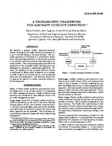
Fig. 1. This figure shows that kernel density estimation after factoring in the image model leads to better estimates. (a) Shown are the data points generated using the 1D image model Y (t) = 10 + 0.2 ∗ (t − 5)2 + N (0, 102 ). To estimate the density f (Y |t = 5) according to Definitions 3 and 4, data points p1 and p2 are moved along straight and curved lines respectively. (b) Shown are the two estimated pdfs, fˆY |t and f˜Y |t to the left and right respectively (ht = 10,hY = 5).

Thus, we will assume kernel K(·) to be separable in the following sense: Let . z = [Y, tT ]T ] denote any data point such that the first coordinate is its intensity component and the rest are its spatial coordinates. Kernel K is separable in the subspaces represented by the intensity and µ spatial coordinates, denoted ¶ 1/hY 01×d . d −1 by DY and Dt = R ª DY . Assuming H = , K(H −1 z) = 0d×1 Ht−1 KY ( hYY )Kt (Ht−1 t). . In (2), values {Yi = Y (ti )}i at locations {ti }i are used to predict the behavior of Y at location u. For the kernel Pn estimate, the expected value of Y conditioned on u is given by, E[Y |u] = i=1 wi (u). Since conditional mean is independent of the regression model, we need to factor the model in Definition 1, into the


5

conditional kernel density estimate in (2). The necessity for doing so is explained using Figure 1(a). At location u = 5 shown on the horizontal axis, E[Y |u] will have a positive bias since most values, Yi , in the neighborhood are larger than the true intensity value at u = 5. The conditional mean will have this bias if the image is not locally linear. In general, the conditional density estimate will be biased wherever the image is not (locally) constant. This effect was noted by Hyndman et. al. [15]. To address this defect, they proposed the following modified kernel estimator which we call the zero bias-in-mean kernel (0-BIMK) conditional density estimator. Definition 4 (0-BIMK Conditional Density Estimator) The zero bias-in. mean kernel (0-BIMK) estimator for the conditional pdf is given by, f˜Y |t (v|u) = Pn 1 −1 [v −Y˜ (ti ); (u − ti )]) such that, Y˜i = I(u) + ²i − ², ²i = i=1 K(H n|H|D Pn Yi − I(ti ), ² = i=1 wi ²i . ˜ |x] = The mean of Y using the above density estimator is, E[Y Pn conditional ˜ w Y = I(x). Thus, the conditional mean of Y computed using the 0-BIMK i=1 i i estimator is guaranteed to be that predicted by the model since the conditional density at any domain point is computed by factoring in the assumed underlying model. In Figure 1(a), we show how the density estimate is constructed using points p1 and p2. While intensity values q1 and q2 (after spatial weighing) are used to find fˆY |t at t = 5, r1 and r2 are used to estimate f˜Y |t . The two estimates are depicted in Figure 1(b) - among them, the latter estimate is clearly a better estimate of 10 + N (0, 102 ). 3.2

0-BIM Parametric Kernel Regression

We are interested in parametric regression models where the regression model, I(t), has the form I(t) = ΘT g(t). Our goal is to estimate the model parameters, ˆ Θ and thus, the regression function, I(t). Let the parameter estimate be Θ. T ˆ ˆ Then, the regression estimate is given by I(t) = Θ g(t). Using Definition 4, the kernel density estimator using the parametric regression model is defined below. Definition 5 (0-BIMK Parametric Density Estimator) The zero bias-inmean kernel (0-BIMK) conditional density estimator, using the parametric regression model I(t) = ΘT g(t) in Definition 1, is given by, n 1 X K(H −1 [v − Y˜ (ti ); (u − ti )]) (3) n|H|D i=1 . . . Pn with Y˜i = g(u)T Θ + ²i (Θ) − ²(Θ), ²i = Yi − g(ti )T Θ and ²(Θ) = j=1 wj ²j (Θ).

. f˜Y |t (v|u, Θ) =

The minimum variance parameter estimator (KMV) for the above density estimate is not a particularly good choice. It is easy to see that the KMV estimate chooses that pdf for the noise process which minimizes the estimated noise variance. This is clearly undesirable if the error pdf is multi-modal. In such a

6


scenario, kernel pdf estimation becomes useful. It provides us with the knowledge that the data is multimodal and assists in choosing the correct mode for the parameter estimate.3 . This prompts the following variant of the ML parameter estimation procedure (one might define other such criteria). ˜ KM L or simDefinition 6 Kernel Maximum Likelihood Parameter Estimator, Θ ˜ ply, Θ, is defined to be that value of Θ which maximizes the likelihood that Y (t) = I(t) when the likelihood is estimated using the 0-BIMK estimator. . ˜ ˜ Θ KML = max fY |t (I(t)|t, Θ) Θ∈Rd

3.3

(4)

˜ Estimation of Θ

˜ is the solution of an unconstrained and differentiable nonlinear program (NLP) Θ which requires global optimization techniques. We introduce now an iterative nonlinear maximization algorithm that is guaranteed to converge to a local maximum for any starting point. The main attractiveness of our algorithm is that it chooses the step size automatically. The convergence result holds if the probability kernel, K(.), has a convex profile (please refer to Chapter 6, [18]). The algorithm can be repeated for several starting points for global maximization (a standard technique for global optimization). We build the proof of convergence using the following two results. Theorem 7 (Least Squares Fit) Given a data sample {[Yi , tTi ]}ni=1 , the Least ˆ LW S in Definition 2 is a Squares fit of the model Y ≈ ΘT g(t), defined by Θ Pn Pn T ˆ solution of the normal equations, i=1 wi g(ti )g(ti ) ΘLS = i=1 wi g(ti )Yi . Lemma 8 Let there be n points, {ti }ni=1 , in Rd , m functions, gi : Rd → R, i = . 1, · · · , m and strictly positive convex weights {wi }ni=1 . Then the matrix A = Pn T 0 i=1 wi (g(ti ) − g(t))(g(ti ) − g(t)) is invertible if and only if there exist n dis√ tinct points, n ≥ n0 ≥ m, such that the set of functions, { wi (g(ti ) − g(t))}m i=1 , is independent over them. d Proof. Let QA be the quadratic Pnform associated with A.2For every y ∈ R , QA (y) . T = y Ay ≥ 0 since QA (y) = i=1 wi ((g(ti ) − g(t)) · y) ≥ 0. Thus, A is positive semidefinite. Hence A is invertible iff it is positive definite. Further, A is positive √ definite iff the set of vectors { wi (g(ti ) − g(t))}i spans Rd . Evidently, this is possible iff there exist n0 distinct points, such that n ≥ n0 ≥ m and the set of √ functions { wi (g(ti ) − g(t))}m ¤ k=1 are independent over such a set. 3

The cost of this generalization achieved by kernel pdf estimation, however, is that one needs to know the scale of the underlying pdf at which it is to be estimated from its samples.


7

Theorem 9 (Parametric Mean Shift using Weighted Least Squares) Let there be n points, {ti }ni=1 , in Rd such that at least m points are distinct. Further, let there be m independent functions, gi : Rd → R, i = 1, · · · , m as in Definition 6. Also, let K be such that K(H −1 z) = KY ( hYY )Kt (Ht−1 t). If KY . has a convex and non-decreasing profile κ, then the sequence {f˜(j)}j=1,2,... = {f˜Y |t (I(t)|t, Θj )}j=1,2,... , of probability values computed at z = (I(t), t) with corresponding parameter estimates {Θj }j=1,2,... defined4 by Θj+1 = argzeroΘ Aj (Θ −Θj ) − bj according to (7) below, is convergent. The sequence {Θj }j=1,2,... converges to a local maximum of {f˜Y |t (I(t)|t, Θ)}. Proof. From Definition (5), . f˜(Θj ) = f˜Y |t (I(t)|t, Θj ) = =

n 1 X K(H −1 [²i (Θj ) − ²¯(Θj ); (u − ti )]) n|H|D i=1

n ²i (Θj ) − ²¯(Θj ) 1 X KY ( )wi hY i=1 hY

Using convexity of the profile κ, defining wi,j = κ0 (− 5

noting all the multiplicative constants by C, we get , f˜(Θj+1 ) − f˜(Θj ) ≥ C

n X

(²i (Θj )−¯ ²(Θj ))2 )wi h2Y

and de-

wi,j {(²ci,j )2 − (²ci,j − (Θj+1 − Θj )T (g(ti ) − g(t)))2 }

i=1

(where,

²ci,j

. . X = (Yi − Y¯ ) − ΘTj (g(ti ) − g(t)) and g(t) = wi g(t))

(5)

i

The above equation shows that the RHS and consequently, the LHS is nonnegative if solution to the following LWS problem exists. n

X . Θj+1 − Θj = argmin wi,j (²ci,j − ΘT (g(ti ) − g(t)))2 Θ∈Rd i=1

From Theorem (7), Θj+1 − Θj must satisfy the following normal equations, n X

wi,j (g(ti ) − g(t))(g(ti ) − g(t))T (Θj+1 − Θj )

i=1

=

n X

wi,j ²ci,j (g(ti ) − g(t)) = ∇Θ f˜(Θj )

(6)

i=1

which has the form Aj (Θj+1 − Θj ) = bj where n

n

i=1

i=1

. X . X Aj = wi,j (g(ti ) − g(t))(g(ti ) − g(t))T ; bj = wi,j ²ci,j (g(ti ) − g(t)) (7) 4 5

y = argzerox g(x) denotes a value of y such that g(y) = 0 P Since f˜(Θj+1 ) − f˜(Θj ) ≥ C n ¯(Θj ))2 − (²i (Θj+1 ) − ²¯(Θj+1 ))2 ) = i=1 wi,j ((²i (Θj ) − ² Pn T 2 C i=1 wi,j (((Yi − Y¯ ) − Θj (g(ti ) − g(t))) − ((Yi − Y¯ ) − ΘTj+1 (g(ti ) − g(t)))2 )

8


Further, Lemma (8) guarantees the existence of a solution. Hence, RHS of (5) =C

n X

wi,j {2²ci,j (Θj+1 − Θj )T (g(ti ) − g(t)) − {(Θj+1 − Θj )T (g(ti ) − g(t))}2 }

i=1

=C

n X

wi,j {(Θj+1 − Θj )T (g(ti ) − g(t))}2 = (∇Θ f˜(j))T (Θj+1 − Θj ) ≥ 0

i=1

. where the equalities follow from (6). The above equation shows that Sf = {f˜(Θj )}j is a nondecreasing sequence. Since the sequence is obviously bounded, it is convergent. RHS of the third equality above also shows that the solution to the normal equations always produces a step which has a positive projection along the gradient of the estimated pdf. By Lemma (8), Aj , j = 1, 2, . . . are fully ranked for all j 0 s. RHS of the second equality above also implies that kδΘj k → 0 . where δΘj = Θj+1 − Θj . . Now, we show that the sequence SΘ = {Θj }j=1,2,... is convergent6 . As the sequence is bounded, it has an isolated (since n is finite) limit point Θ∗ . Since δΘj → 0, given small enough r, ², 0 < r < r + ² and open balls B(Θ∗ , r), B(Θ∗ , r + ²), there exists an index J1 such that for all j > J1 , kδΘj k < ², Θ∗ . is the only limit point in B(Θ∗ , r + ²) and the set U = {Θ|Θ ∈ B(Θ∗ , r + ²) ∩ B c (Θ∗ , r), Θ ∈ S} in non-empty. U has finite items, let their maximum value be MU . Further, as Sf is strictly increasing, there exists an index J2 such that for all j > J2 , f˜(Θj ) > MU . We define J = max(J1 , J2 ). Then, for any j > J, Θj ∈ B(Θ∗ , r) ⇒ Θj+1 ∈ B(Θ∗ , r) since B(Θ∗ , r) ∪ B(Θj , δΘj ) ⊂ B(Θ∗ , r + ²) and Θj+1 ∈ / U . Further, δΘj → 0 ⇒ bj = ∇Θ f˜(Θj ) → 0. Hence, Θ∗ is a point of local maximum for f˜(·). ¤ Thus, Theorem (9) guarantees a solution to the kernel maximum likelihood problem in the sense that given any starting point, we would converge to a local maximum of the parametric kernel likelihood function. However, at each iteration step, a weighted least squares problem needs to be solved that requires matrix inversion. Further, it is required that in the limit, the matrix Aj stays positive definite. This condition need not always be satisfied. In the next theorem, we provide a way to bypass this condition. Theorem 10 (Parametric Mean Shift using Gradient Descent) Let there be n points, {ti }ni=1 , in Rd such that at least m points are distinct. Further, let there be m independent functions, gi : Rd → R, i = 1, · · · , m in terms of ˜ KM L as given in Definition 6. Also, let K be such which we want to find Θ that K(H −1 z) = KY ( hYY )Kt (Ht−1 t). If KY has a convex and non-decreasing . profile κ, then the sequence {f˜(j)}j=1,2,... = {f˜Y |t (I(t)|t, Θj )}j=1,2,... of probability values computed at z = (I(t), t) with corresponding parameter estimates {Θ}j=1,2,... , defined by Θj+1 = Θj + kj ∇Θ f˜(Θj ) in (8), is convergent. The sequence {Θj }j=1,2,... converges to a local maximum of {f˜Y |t (I(t)|t, Θ)}. 6

We gratefully acknowledge Dr. Dorin Comaniciu’s assistance with the proof.


9

Proof. From (5), f˜(Θj+1 ) − f˜(Θj ) ≥ C

n X

wi,j (²ci,j )2 − (²ci,j − (Θj+1 − Θj )T (g(ti ) − g(t)))2

i=1

Now, we take the next step in the direction of the gradient, i.e., we seek some kj > 0 such that Θj+1 = Θj + kj ∇Θ f˜(Θj ) and kj is the solution of, kj = argmin

n X

k

wi,j (²ci,j − k

i=1

n X

wl,j ²cl,j g c (tl )T g c (ti ))2

l=1

Solving for kj , we get, Pn k i=1 wi,j ²ci,j g(ti )k2 N (kj ) 1 Pn kj = Pn =: ≥ Pn >0 c g(t )i2 D(k ) w hg(t ), w ² w kg(ti )k2 j i,j i l,j l i,j i=1 l=1 i=1 l,j Hence, RHS of (8) = C

n X

" wi,j

²ci,j 2

−

i=1

(²ci,j

− kj

n X

# wl,j ²ci,j g(tl )T g(tl ))2

l=1

N (kj )k∇Θ f˜(Θj )k2 C =C = C(Θj+1 − Θj ) · ∇Θ f (Θj ) = kΘj+1 − Θj k2 ≥ 0 D(kj ) kj . This implies the convergence of Sf = {f˜(Θj )}j and that kδΘj k → 0 as in the . proof for Theorem 9. The convergence of SΘ = {Θj }j=1,2,··· to a local maximum similarly follows. ¤ The gradient descent algorithm is more stable (albeit slower) since it does not require matrix inversion. Hence, we use this algorithm for applications in Section 5.

4

Empirical Validation

We tested the robustness of our algorithm empirically and compared its statistical performance with (a) the least squares (LS) method, and, (b) the least trimmed squares (LTS) method. The comparison to LS was done since it is the most popular parameter estimation framework apart from being the minimumvariance unbiased estimator (MVUE) for additive white Gaussian noise (AWGN), the most commonly used noise model. Further, our algorithm is a re-weighted LS (RLS) algorithm. LTS [19] was chosen since it is a state-of-the-art method for robust regression. We note here that LS is not robust while LTS has a positive breakdown value of ([(n-p)/2] + 1)/n [19]. In computer vision, one requires robust algorithms that have a higher breakdown value [20]. Redescending Mestimators (which the proposed formulation yields) are shown to have such a property. Thus, theoretically, they are more robust then either of the estimators

10


Table 1. LS, LTS and KML estimates for (a, b, c). Ii = ax2i + bxi + c + ²i . {²i } are i.i.d. Gaussian and i.i.d. log-normal with parameters (0, σ 2 ) for experiments in left and right columns respectively. Ground-truth values are (a, b, c) = (0.135, 0.55, 1.9). Mean and standard deviation of the estimated values for 1000 experiments are presented for each estimator - LS, LTS and KML, in rows 1, 2, and 3, respectively. KML performs better for log-normal while LTS and LS perform better for gaussian noise.

σ 1 5 9 13

a 0.135 0.135 0.135 0.135

λ 1 5 9 13

a 0.135 0.135 0.135 0.135

σ 1 5 9 13

a 0.135 0.135 0.135 0.135

LS - Gaussian noise Mean Standard Deviation b c a b c 0.550 1.907 0.0001 0.0036 0.1516 0.549 1.952 0.0007 0.0165 0.7474 0.549 1.853 0.0012 0.0308 1.3658 0.548 1.951 0.0017 0.0449 1.9375 (a) LTS - Gaussian noise Mean Standard Deviation b c a b c 0.549 1.905 0.0002 0.0036 0.1881 0.547 2.005 0.0007 0.0177 0.8838 0.551 2.000 0.0011 0.0292 1.2843 0.550 2.003 0.0015 0.0335 1.7416 (c) KML - Gaussian noise Mean Standard Deviation b c a b c 0.549 1.904 0.0002 0.0036 0.2697 0.547 1.960 0.0008 0.0166 1.0517 0.546 1.950 0.0015 0.0311 1.8904 0.544 1.951 0.0021 0.0481 2.6815 (e)

LS - log-normal noise Mean Standard Deviation σ a b c a b c 1 0.135 0.550 1.917 0.0004 0.0098 0.4016 2 0.135 0.555 1.729 0.0063 0.1369 7.6999 3 0.140 0.194 6.673 0.2862 6.7165 2.36e2 4 0.762 1.605 -8.7e2 2.00e1 3.68e2 3.05e4 (b) LTS - log-normal noise Mean Standard Deviation λ a b c a b c 1 0.135 0.549 1.810 0.0005 0.0148 0.6224 2 0.135 0.550 1.996 0.0007 0.0179 0.8286 3 0.135 0.549 1.963 0.0009 0.0257 1.0629 4 0.135 0.548 1.973 0.0014 0.0380 1.7173 (d) KML - log-normal noise Mean Standard Deviation σ a b c a b c 1 0.135 0.549 1.931 0.0004 0.0083 0.4570 2 0.135 0.548 1.927 0.0007 0.0164 0.7446 3 0.135 0.548 1.916 0.0007 0.0198 0.8184 4 0.135 0.547 1.992 0.0011 0.0204 1.5543 (f)

described above. Nonetheless, it is useful to benchmark the performance of the proposed estimator with the above two estimators. For ease of comparison, we used a 1-D data set as our test bed (Table 1). Intensity samples were generated using the equation I0 (x) = ax2 + bx + c at unit intervals from x = −50 to x = 50. To test the noise performance, we added uncorrelated noise from a noise distribution to each intensity sample independently. We used Gaussian and two-sided log-normal distributions as the noise density functions. We tested the performance at several values of the variance parameter associated with these distributions. At each value of variance, we generated 1000 realizations and calculated the bias and the variance of the two estimators. The Gaussian distribution was chosen as the LS estimator is the minimum variance unbiased estimator (MVUE) for AWGN noise while the log-normal distribution was chosen to simulate outliers. We present the results in Table 1: results for i.i.d. Gaussian noise are presented in the left column and for i.i.d. log-normal


11

noise are presented in the right column. The ground-truth values are a = 0.135, b = 0.55 and c = 1.9. The results show that the performance of the proposed estimator is better than the LTS and the LS estimators when the number of outliers are large (log-normal noise). In case the noise is AWGN, standard deviation of the proposed estimator stays within twice that of the LS estimator (which is the MVUE). However, the proposed algorithm has a better breakdown value than either of the two estimators . Further, the proposed estimator is easy to implement as a recursive least squares (RLS) algorithm, and, in our simulations, it was an order of magnitude faster than the LTS algorithm.

5

Applications

The theoretical formulation derived in the previous sections provides a robust mechanism for parametric (global) or semi-parametric (local) image regression. This is achie-ved via a parametric representation of the image signal coupled with non-parametric kernel density estimation for the additive noise. As a consequence, the proposed estimation framework can be used for the following tasks: (A1) Edge preserving denoising of images that can be modelled (locally or globally) using the linear parametric model in Definition 1. (A2) Further, since the KML Estimation framework admits a multimodal error model, the framework can be used to partition data generated from a mixture of sources, each source generating data using the aforementioned parametric model (in such a case, we use Ht → ∞. In other words, spatial kernel is assumed identically equal to one). Thus, the proposed framework provides a systematic way of doing Hough Transforms. Indeed, Hough Transform is the discretized version of f˜Y |t (ΘT g(t)) if HY → 0 and Ht → 0. To illustrate an application of the proposed estimation framework, we apply it to the task of range image segmentation. As test images, we use the database7 [21] generated using the ABW structured light camera. The objects imaged in the database are all piecewise linear and provide a good testbed for the proposed estimation framework. Let the range image be denoted by Y (t). Then, for each t in the image domain D, the range may be represented as Y (t) = h[tT 1]T , Θ(t)i + ²(t) where . Θ(t) ∈ SΘ = {Θ1 , · · · , ΘM } such that there are M unknown planar regions in the range image. The task of planar range image segmentation is to estimate the set SΘ and to find the mapping, T : D → SΘ . The algorithm used for segmentation has following steps: (1) Estimate8 lo˜ cal parameters, Θ(t) for each t. This also provides an edge-preserved de-noised ˜ ˆ range image (I(t)). (2) Sort Θ(t)’s in descending order of likelihood values, T T ˜ ˜ ˜ fY |t (h[t 1] , Θ(t)i). (3) Starting with the most likely Θ(t), estimate the pa˜ p ) of the largest (supported) plane (spatial bandwidth matrix rameters (say, Θ 7

8

Range Image Databases provided on the University of South Florida website http://marathon.csee.usf.edu/range/DataBase.html. KML estimation requires specification of the bandwidth parameters. These are handselected currently although they can be estimated akin to [17].

12


∞ for global estimation). Since kernel maximum likelihood function can have several local minima, sorting has the effect of avoiding these local minima. ˜ p (t)i) Next, remove the data points supported by this plane (f˜Y |t (h[tT 1]T , Θ greater than a threshold) from the set of data points as well as from the sorted list. (4) Choose the next (remaining) point from the sorted list and fit the next largest plane to the remaining data points. (5) Iterate Step (4) N times (N >> M , we choose N = 100) or until all data points get exhausted. (6) Discard the planes smaller than k pixels (resulting in N1 planes), and con. ˜ ˜ struct the set SΘ = {Θ 1 , · · · , ΘN1 }. (7) Reclassify all data points based on the likelihood values, i.e. the function T (·) is initially estimated to be T (t) = ˜ p (t)i |(t), Θ ˜ i ). (8) Repeat step (6). (9) Refine bounargmaxi∈1...N1 f˜Y |t (h[tT 1]T , Θ daries based on the geometric reasoning that all intersecting planes produce straight lines as edges (refer to Chapter 6, [18]).

(a)

(b)

(c)

(d)

Fig. 2. Results for ABW test images 27 (row 1) and 29 (row 2). (a) Original range ˆ image, (b) reconstructed range image I(t) (locally planar assumption), (c) extracted planar segments, (d) Final segmentation after geometric boundary refinement. Edges are superimposed on the intensity images.

In Figure 2, we show segmentation results on two9 range images from the ABW data set. The range values in column (a) properly belong to piecewise planar range data. The range data is missing in the (black) shadowed regions. We treat these regions as planar surfaces that occlude all neighboring surfaces. ˆ The estimated locally linear surface (output of step 1, I(t)) is shown in column 9

More results will be included in the two extra pages allowed for the final manuscript.


13

(b). To better illustrate the results of KML estimation, we reproduce a scan line in Figure 3(a). Note, in Figure 3(b), that occluding edge (discontinuity in the range data) is well preserved while denoising within continuous regions takes place as expected. This illustrates that the kernel maximum likelihood estimation preserves large discontinuities while estimating image parameters in a robust fashion. At the same time, locally estimated planar parameters are close to true values (refer to Figure 3(c) and the caption). After planar regions are extracted in step (7), we show the results in Figure 2(c). Here, the brightness coding denotes different label numbers. We see that very few spurious regions are detected - this validates the robustness of global parameter estimation framework since we fit global planes to the data and iteratively remove data points supported by the planes. The goodness of the estimated plane parameters now allows us to carry out the geometric boundary refinement step as we can now estimate the corner and edge locations as detailed above. The final result after this is depicted in Figure 2(d). As one can see, the estimated segmentation is near perfect. To see that our results are better than several well-known range image segmentation algorithms, please compare them visually with those presented in Hoover et al [21].

240

70

120

50

45 60

220

100 40

50

35

200

80 30 40

180

60

25

30 20 160

40 15

20

10 140

20

10

5

120

(a)

0

50

100

150

(b)

200

250

300

0

0.08

0.1

0.12

0 −0.4

−0.3

−0.2

0 130

135

140

(c)

Fig. 3. (a) ABW test image 29. (b) Noisy and reconstructed range image (locally planar assumption) values are shown, along the scan line in (a), depicting robustness to discontinuities. (c) Estimated histogram of computed planar parameters for each data point of the leftmost object plane are shown. True image model : I = 0.095y − 0.294x + 136.35.

6

Conclusions

In this paper, we presented a robust maximum likelihood parameter estimation framework by modelling the image with a linear parametric model and additive noise using kernel density estimators. The resulting estimator, the KML Estimator, is a redescending M-estimator. This novel approach provides a link between robust estimation of parametric image models and nonparametric density models for additive noise. We also provided a solution to the resultant nonlinear optimization problem and proved its convergence. Finally, we apply our framework to range image segmentation.

14


References 1. Huber, P.J.: Robust regression: Asymptotics, conjectures and monte carlo. The Annals of Statistics 1 (1973) 799–821 2. Yohai, V.J., Maronna, R.A.: Asymptotic behavior of M-estimators for the linear model. The Annals of Statistics 7 (1979) 258–268 3. Koenker, R., Portnoy, S.: M-estimation of multivariate regressions. Journal of Amer. Stat. Assoc. 85 (1990) 1060–1068 4. Chu, C.K., Glad, I.K., Godtliebsen, F., Marron, J.S.: Edge-preserving smoothers for image processing. Journal of the American Statistical Association 93 (1998) 526–541 5. Hillebrand, M., Muller, C.H.: On consistency of redescending Mkernel smoothers. unpublished manuscript - http://www.member.unioldenburg.de/ch.mueller/publik/neuarticle5.pdf 9 (2000) 1897–1913 6. Ayer, S., Sawhney, H.: Layered representation of motion video using robust maximum likelihood estimation of mixture models and MDL encoding. Computer Vision, Int’l Conf. (1995) 777–784 7. Black, M.J., Jepson, A.D.: Estimating optical flow in segmented images using variable-order parametric models with local deformations. PAMI, IEEE Trans. 18 (1996) 972–986 8. Kumar, R., Hanson, A.R.: Robust methods of estimating pose and a sensitivity analysis. Image Understanding, CVGIP (1994) 9. Liu, L., Schunck, B.G., Meyer, C.C.: On robust edge detection. Robust Computer Vision, Int’l Workshop (1990) 261–286 10. Mirza, M.J., Boyer, K.L.: Performance evaluation of a class of M-estimators for surface parameter estimation in noisy range data. IEEE Trans., Robotics and Automation 9 (1993) 75–85 11. Stewart, C.V.: Robust parameter estimation in computer vision. SIAM Reviews 41 (1999) 513–537 12. Tomasi, C., Manduchi, R.: Bilateral filtering for gray and color images. Computer Vision, 6th Intl. Conf. (1998) 839–846 13. Barash, D., Comaniciu, D.: A common framework for nonlinear diffusion, adaptive smoothing, bilateral filtering and mean shift. Image and Video Computing (2003) 14. Boorngaard, R., Weijer, J.: On the equivalence of local-mode finding, robust estimation and mean-shift analysis as used in early vision tasks. Pattern Recognition, 16th Intl. Conf. 3 (2002) 927–930 15. Hyndman, R.J., Bashtannyk, D.M., Grunwald, G.K.: Estimating and vizualizing conditional densities. Journal of Comput. and Graph. Statistics 5 (1996) 315–336 16. Chen, H., Meer, P.: Robust computer vision through kernel density estimation. Computer Vision, 7th Euro. Conf. 1 (2002) 236–250 17. Singh, M.K., Ahuja, N.: Regression-based bandwidth selection for segmentation using Parzen windows. Computer Vision, 9th Intl. Conf. (2003) 2–9 18. Singh, M.K.: Image Segmentation and Robust Estimation Using Parzen Windows. University of Illinois at Urbana-Champaign. Ph.D. Thesis (2003) 19. Rousseeuw, P.J., Van Driessen, K.: Computing LTS Regression for Large Data Sets. University of Antwerp. Technical Report (1999) 20. Mizera, I., Muller, C.H.: Breakdown points and variation exponents of robust M-estimators in linear models. Annals of Statistics 27 (1999) 1164–1177 21. Hoover, A., J.-B., G., Jiang, X., Flynn, P.J., Bunke, H., Goldgof, D.B., Bowyer, K.K., Eggert, D.W., Fitzgibbon, A.W., Fisher, R.B.: An experimental comparison of range image segmentation algorithms. PAMI, IEEE Trans. 18 (1996) 673–689