A Robust Feature Extraction for Automatic Speech Recognition in Noisy Environments Carlos Lima, Luís B. Almeida* and João L. Monteiro Department of Industrial Electronics of University of Minho, Portugal {carlos.lima, joao.monteiro}@dei.uminho.pt *Department of Electrical and Computers Engineering, IST, Technical Univ. of Lisbon, Portugal
[email protected]
Abstract This paper presents a method for extraction of speech robust features when the external noise is additive and has white noise characteristics. The process consists of a short time power normalisation which goal is to preserve as much as possible, the speech features against noise. The proposed normalisation will be optimal if the corrupted process has, as the noise process white noise characteristics. With optimal normalisation we can mean that the corrupting noise does not change at all the means of the observed vectors of the corrupted process. As most of the speech energy is contained in a relatively small frequency band being most of the band composed by noise or noise-like power, this normalisation process can still capture most of the noise distortions. For Signal to Noise Ratio greater than 5 dB the results show that for stationary white noise, the normalisation process where the noise characteristics are ignored at the test phase, outperforms the conventional Markov models composition where the noise is known. If the noise is known, a reasonable approximation of the inverted system can be easily obtained performing noise compensation still increasing the recogniser performance.
1. Introduction Noise robustness can be accomplished either at the feature representation level using robust parameterisation or at the model compensation level. Generally, in the feature analysis process, only a lightly knowledge about the noise characteristics is needed. Some approaches maintain that the corrupting noise is by nature unknown, thus it is meaningless trying to compensate for it. Therefore, the search for a robust speech representation that diminishes the distortions caused by the environment seems to be the most promising solution to deal with noise conditions. Noise pre-filtering [1] [2], projection based distortion measures [3], vector space mapping [4] [5], all pole modelling of the autocorrelation sequence [6] [7] [8] [9] and [10], speech representation motivated by the human auditory system knowledge (Perceptually Linear Prediction analysis (PLP)) [11] [12], and more recently, complementing the PLP technique with a band-pass filter (RASTA-PLP) [13], have been the techniques more successful used for the robust representation of the speech.
However, in spite of the effort dedicated for these last years in the field of the robust parameterisation, conceiving systems with acceptable performance in environments for which they were not trained has been far too difficult. Techniques based on the noise modelling (compensation) seem more promising than those based on the robust parameterisation, once it seems extremely difficult to conceive a system of signal processing whose outputs stay unchangeable from the clean to the noisy speech processing. Those techniques assume that even being the corrupting noise by nature unknown it can be compensated. Even assuming this as a reasonable approach those techniques frequently present two main limitations: 1) Modelling conveniently the noise increases the computation, slowing down the recognition process. 2) Usually does not exist isolated noise samples at least in sufficient amounts to train the noise model. Therefore, the accuracy of this model can commit the effectiveness of the speech recogniser even in relatively quiet environments. In environments characterised by a strong non-stationary nature noise compensation becomes a much more difficult task. Among others, these limitations encourage the search for a robust speech representation, given that this approach becomes potentially more promising than the techniques that try to compensate the unknown and frequently non-stationary corrupting process. The Mel Frequency Cepstral coefficients (MFCC) are more robust against noise than some other classical features, while the PMC technique [15] compensates the noise in the MFCC domain. However, the suggested spectral normalisation is more robust against noise than the MFC coefficients if the noise is additive, has white noise characteristics and normal distribution.
2. Spectral Normalisation This spectral normalisation is motivated by the fact that the additive noise is not a narrow band noise, thus its spectrum is reasonably dispersed in frequency and the goal is preserving as much as possible the speech features against noise. The process consists in a division of the frequency band in sub-bands given that usually a very fine detail in frequency is not required for speech recognition applications. The method is based on the power spectral density components and consists in dividing the speech power inside each sub-band by the total short-time speech power. The power in each sub-band is obtained summing
the components of the power spectral components inside the subband. All the sub-bands have the same number of spectral components and any spectral component is shared by different sub-bands thus, avoiding increases of statistical dependence between sub-bands (feature components). The background noise contributes to increase simultaneously the sub-band and total power, which contributes for stabilising the feature values. To best understand this reasoning, consider Si denoting the speech power in sub-band i and S denoting the short time speech power of the considered segment. Similarly, let Ni, N denote the power of the noise in sub-band i and the short time noise power, respectively. So, the ith component of the observation vector for clean and noisy speech are given respectively by
ci =
Si S
,
ci =
Si + N i S+N
(1)
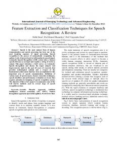
Figure 1 shows the clean speech and noisy speech spectral power normalisation features for 240 ms of the word “zero” where each sub-band has 16 power spectral components. The SNR is 0 dB.
related by the quotient l/L. Using these considerations the calculation of the shift vector imposed by the environment is accomplished by subtracting equations (1) and becomes [14]
Si l 1 − k , k = 1+ Ci ( N ) = − S L k
Di =
0.4 0.35 0.3
0.2 0.15 0.1 0.05 0
0
5
10
15
20
25
30
35
40
45
50
Sub-band Figure 1. White noise effect in the power spectrum density normalization domainin the beginning of digit “zero”. Dashed line represents noisy speech features.
If the noise has white noise characteristics the environment will shift the clean speech vector by a noise dependent vector Ci(N), which can be calculated by subtracting equations (1)
S + N i Si − Ci ( N ) = i S+N S
(4)
Zi − X i Xi
where Zi is the ith component of the observation vector for noisy speech and Xi has the same meaning but for clean speech. It is evident by comparing figure 1 and figure 2 that the “peaked” spectral regions of the clean speech are more robust against additive white noise than the rest of the band. Additionally the proposed normalisation shows more robustness (less deviation in the features) for all the frequency sub-bands. 300
250
200
150
100
50
(2)
0
-50 0
If the noise is stationary then its short time power equals its long time power. For the speech this is not true due to its nonstationary property, but as an approximation we will consider that the short time speech signal power equals the long time speech signal power. Under this constraint S and N can be related by the signal to noise ratio (SNR). Therefore the next expression holds
1 S + N = S 1 + SNR 10 10
10
SNR 10
Equation (4) shows that if the speech has a flat power spectrum density, the means of Ci(N) become null given that Si/S equals l/L. Thus, this normalisation process becomes optimal in the sense that the environment does not affect the means of the speech features. This means that this normalisation procedure provides some noise robustness to unvoiced speech segments, where neither the speech nor the noise are spectrally well defined. Figure 2 shows the relative deviation caused by the environment (additive white noise at 0 dB) in the suggested power spectrum normalisation domain and in the power spectrum density domain. The relative deviation was computed as
0.45
0.25
1
(3)
Let l, the number of components in each sub-band and L the FFT length. Then N and Ni, considering flat noise spectrum, are
5
10
15
20
25
30
35
40
45
50
Sub-band Figure 2. Relative deviation caused by additive white noise at 0 dB at the beginning of digit “zero” when working in the power spectral density domain (normal line) and in the power spectral density normalisation domain (dashed line).
3. Markov models composition in the spectral normalisation domain The basic idea of the HMM composition is to recognise concurrent signals simultaneously. Parallel HMMs are used to model the concurrent signals and the composite signal is modelled as a function of their combined outputs. To perform Markov models composition one has to know the composite
signal distribution and the statistical model of the corrupting environment. 1) Distribution of the composite signal (noisy speech): Usually the corrupting Gaussian additive white noise process is considered in the time domain. As the Fourier Transform is a linear operation then the distribution is maintained from time to frequency domain. It is well known from the statistics theory that if a random variable has a Gaussian distribution then the square of its modulus (power spectral density) has a chi-square distribution with two degrees of freedom, also known by exponential distribution. As the speech and noise are considered additive in the time domain, the additivity is maintained in the power spectrum density (PSD) domain. The clean speech is modelled as Gaussian in the PSD domain and the distribution of the noisy speech becomes the convolution between a Gaussian and an exponential function. Reference [14] shows that the noisy speech distribution is as follows
f z ( z) =
e
−
4 λz − 4 λµ y − 2σ y2 4 λ2
2λ
adequate, however, for smooth distributions a number as low as 5 can be used. In our case we have 16 random variables and no smooth distributions, so a considerable difference between the real and approximated function can be expected. This difference is shown in figure 4 for λ=10. However, in real situations λ is greater, (order of 107 at 10dB), the variance is in order of the square of λ and the Gaussian function fits best to the function defined by equation (6), what is expected by the inspection of figure 4.
λz − λµ − σ 2 y y 1 + erf 2σ y2 λ (5)
where the y vector refers to the clean speech signal, λ is the parameter of the exponential distribution and erf stands for the well known error function. However, to reduce the observed vector dimensionality when working in the spectral density space it is commun grouping by sum some contiguous components. The number of components considered must be a compromise between the training database size and the frequency resolution required. In our case we used 16 components in each sub-band. Therefore equation (5) holds for the noisy speech distribution, and it would be still necessary to develop the distribution of the sum of 16 random variables each one with the distribution given by this equation. As equation (5) is complex to handle by convolution, an easier solution is to develop the probability density function of the sum of 16 exponential distributed random variables (noise in sub-bands) and perform the convolution of this function with a Gaussian function which models the sum of 16 spectral components of the clean speech. By mathematical induction it is easy to prove [14] that the distribution of the sum of 16 random independents and identically distributed variables is
w w15 exp− λ U ( w) fW ( w) = 15!λ16
(6)
The integral of convolution between the above equation and a Gaussian function becomes very difficult to calculate due to the w15 term. Using the Central Limit Theorem equation (6) can be approximated by a Gaussian function with mean equal to 16λ and variance equal to 16λ2. The nature of the Central Limit theorem approximation and the required number of variables for a specified error bound, depend on the form of the densities of the summed random variables. For most applications a number of 30 random variables is
Figure 4. Approximation of the sum of 16 random i. i. d. variables with λ=10, by a Gaussian function.
Under this approximation the noisy speech distribution becomes
f z ( z) =
1 4 2π σ y2 + 16λ 2
−
e
( z − µ y −16 λ ) 2 2 (σ y2 +16 λ2 )
(7)
2) Noisy speech distribution in the spectral normalisation space: As shown above the noise can be approximately Gaussian modelled in the sub-band PSD domain and so, the noisy speech has also a Gaussian distribution. Similarly, we can consider that if the clean speech spectral normalisation can be Gaussian modelled then the noisy speech spectral normalisation follows also a Gaussian distribution. So Ci(N) has a Gaussian distribution given the distribution of the speech features is Gaussian and all the other terms involved in the equation (2) are considered constants for white noise. The knowledge of the Ci(N) statistics is then reduced to the knowledge of its mean and variance. Using equation (4) the next expression holds for the mean
S + Ni 1 Si l 1 − k E i = E − S+N k S L k
(8)
where k is given in equation (4). The variance of the corrupted process can be similarly calculated, considering white noise and that each sub-band is composed by summing 16 power spectral density components
Si S + Ni 1 k −1 var i = 2 var + 16 k S S+N k (9)
2
Updating the clean speech HMM distributions according to equations (8) and (9), that is, performing Markov model composition for stationary white noise in the spectral normalisation domain, the recognition accuracy was increased as it can be seen in table 1.
4. Experimental Results The proposed algorithm was tested in an Isolated Word Recognition system using Continuous Density Hidden Markov models. The database of isolated words used for training and testing is from AT&T Bell. The used speech was acquired under controlled environmental conditions band-pass filtered from 100 to 3200 Hz, sampled at a 6.67 kHz and analysed in segments of 45 ms duration at a frame rate of 66.67 windows/sec. Only the decimal digits were used. The noise has white noise characteristics, is speech independent and computationally generated at various SNR as shown in table 1. The goal is to compare the performance of the proposed and contemporary speech robust features. Some of these robust features are the OSALPC (One-Sided Autocorrelation Linear Predictive Coding), the conventional cepstrum with liftering (CEPS + liftering) and the well known MFCC (Mel-Frequency Cepstral Coefficients. In table 1 MMC stands for conventional Markov model composition in the power spectrum density domain, Norm. stands for the proposed normalisation procedure and N. + MMC stands for Markov model composition in the proposed power normalisation domain. Table 1 shows that the suggested spectral normalisation features are more effective against additive white noise than some robust features used nowadays. For SNR greater than or equal to 5 dB the spectral normalisation outperforms the conventional Markov model composition (MMC) when the noise parameters are learned from the periodogram method in a data segment of 100ms without speech. As in the Parallel Model Combination, the distortion can be integrated (compensated) in the composite model increasing thus the recogniser performance. On the first six entries of the table 1 all the features are 8 static, energy and dynamic features excepting * (12 static + energy + dynamics) and ** (13 static + energy + dynamics). Table 1 – Performance of the spectral normalisation SNR (dB) 15 10 5 0 -5 LPC 56.5 39.5 30 16.2 OSALPC 98.25 92 65.75 32.2 CEPS * 97.5 95 72 34.5 +liftering 98.25 95 75.25 39 MFCC ** 97.75 94.7 72.25 37.5 OSALPC* 98.5 96.2 74.25 32.5 MMC 98 96.7 92.5 91 78.5 Norm. 98.5 97.7 93.75 88 42.5 N.+ MMC 99.5 98.7 97.25 92.2 84.75
5. Discussion The main advantage of this normalisation process is the recognition performance obtained when no knowledge of the noise statistics exists. The proposed normalisation will be optimal if the corrupted and the noise process have both white noise characteristics. This can mean that also unvoiced speech
segments (speech segments without voiced regions) are more preserved against additive noise. This makes some sense; since the spectral regions with less energy are more corrupted thus, need more robustness. For high Signal to Noise Ratios the spectral normalisation, where the distortion is ignored at the test phase, outperforms the Markov model composition where the distortion is learned from a small amount of isolated noise samples and incorporated into the system. If isolated noise samples exist, the noise can be estimated and this knowledge can be incorporated into the system increasing the recogniser performance.
References [1] Boll, S.F. (1979). Suppression of acoustic noise in speech using spectral subtraction, IEEE Trans. Acoust, Speech, Signal Processing, Vol. ASSP–27, n.º 2, pp. 113–120. [2] Compernolle, D.Van. (1989). Noise adaptation in a hidden Markov model speech recognition system. Comput, Speech, Language, Vol. 3, pp.151–167. [3] Mansour, D. and Juang, B.H. (1989). A family of distortion operators based on projection operation for robust speech recognition. IEEE Trans. Acoust., Signal Processing, pp. 1659– 1671. [4] Gish, H., Chow, Y. and Rohlicek, J.R. (1990). Probabilistic vector mapping of noisy speech parameters for HMM word spotting. In Proc. Int. Conf. Acoust., Speech, Signal Processing, pp. 117–120. [5] Juang, B.H. and Rabiner, L.R. (1987). Signal restoration by spectral mapping. In Proc. Int. Conf. Acoust., Speech, Signal Processing, pp. 2368–2371. [6] Mansour, D. and Juang, B. (1988b). The short-time modified coherence representation and its application for noisy speech recognition. In. ICASSP, pages 525- 528. [7] Mansour, D. and Juang, B. (1989a), The short-time modified coherence representation and its application for noisy speech recognition. IEEE Trans., ASSP, ASSP – 37 (6) : 795 – 804. [8] Hernando, J. and Nadeu, C. (1991). A comparative study of parameters and distances for noisy speech recognition. In EUROSPEECH, pages 91- 94. [9] Hernando, J., Nadeu, C. and Lleida, E. (1992). On the AR modelling of the one-sided autocorrelation sequence for noisy speech recognition. In ICSLP, pages 1593 - 1596. [10] Hernando, J., Nadeu, C. (1994). Speech recognition in noisy car environment based on OSALPC representation and robust similarity measuring techniques. In ICASSP, pages II.69 – II.72. [11] Hermansky, H., Hanson, B. and Wakita, H. (1985). Low– dimensional representation of vowels based on all-pole modelling in the psychophysical domain. Speech Communication, 4(13):181-187. [12] Hermansky, H. (1990). Perceptual Linear Predictive (PLP) analysis of speech. J. Acoust. Soc. Am., 87(4): 1738–1752. [13] Hermansky, H., Morgan, N. Bayya, A. and Kohn, P. (1991). Compensation for the effect of the communication channel in auditory like analysis of Speech (RASTA–PLP). In EUROSPEECH, pages 1367–1370. [14] Lima, Carlos. Speech Recognition in non-Stationary Environments. Ph. D. Thesis to submit in the Department of Industrial Electronics of University of Minho (Portugal) [15] Gales, M. and Young, S. (1994). Parallel model combination on a noise corrupted resource management task. In ICSLP, pages 255-258.