word error rate: improvements of up to 14% on the small- vocabulary task and ..... max. likelihood training using Viterbi approximation. The baseline system has ...
Extraction Methods of Voicing Feature for Robust Speech Recognition Andr´as Zolnay, Ralf Schl¨uter, and Hermann Ney Human Language Technology and Pattern Recognition Chair of Computer Science VI RWTH Aachen – University of Technology 52056 Aachen, Germany
fzolnay,
g
schluter, ney @informatik.rwth-aachen.de
Abstract In this paper, three different voicing features are studied as additional acoustic features for continuous speech recognition. The harmonic product spectrum based feature is extracted in frequency domain while the autocorrelation and the average magnitude difference based methods work in time domain. The algorithms produce a measure of voicing for each time frame. The voicing measure was combined with the standard Mel Frequency Cepstral Coefficients (MFCC) using linear discriminant analysis to choose the most relevant features. Experiments have been performed on small and large vocabulary tasks. The three different voicing measures combined with MFCCs resulted in similar improvements in word error rate: improvements of up to 14% on the smallvocabulary task and improvements of up to 6% on the largevocabulary task relative to using MFCC alone with the same overall number of parameters in the system.
1. Introduction Standard state-of-the-art automatic speech recognition systems use spectral (e.g. Mel Frequency Cepstral Coefficients, MFCC) representation of the speech signal. However, these representation techniques are not robust to acoustical variation like background noise, speaker change etc. Word error rate can increase considerably under real life conditions. A possible way to increase robustness of speech recognition could be finding representative features of the speech signal and corresponding robust extraction methods. In this work we investigated the voicing feature. Voiced sounds are produced by quasi periodic oscillation of the vocal chords. A feature value explicitly measuring the state of the vocal chords can lead to better discrimination of voiced and unvoiced sounds and consequently to better recognition results. The first related studies go back to rule based speech recognition where voiced-unvoiced detection was used as one of different acoustical features, see Chapter “The Speech Signal” in [1]. In [2] experiments with autocorrelation based voicing measure are reported. Standard MFCCs with 1st and 2nd derivatives are used as acoustic feature vector augmented by the voicing measure and its 1st and 2nd derivatives. In [3] fundamental frequency and a voicing measure is combined with standard MFCCs using linear discriminant analysis (LDA). In this paper, we describe implementation issues and the evaluation of three different voicing extraction methods: 1) harmonic product spectrum based, 2) autocorrelation based, and 3) average magnitude difference based, see Chapter “Pitch Detection” in [4]. The extraction methods produce
a measure of voicedness for each time frame. The voicing measures were combined with the standard MFCC features using linear discriminant analysis. Experiments showed similar improvements in word error rate (WER) for the three extraction methods: relative improvements of up to 14% on smallvocabulary task and relative improvements of up to 6% on largevocabulary task due to one additional voicing feature. The rest of the paper is organized as follows. In Section 2, the baseline MFCC signal analysis is described. In Section 3, the three different extraction methods are derived. Experiments will be presented in Section 4, followed by a summary in Section 6.
2. Baseline Signal Analysis In this section, the standard MFCC signal analysis component of our speech recognition system is described. First we perform a preemphasis of the sampled speech signal. Every 10ms, a Hamming window is applied to preemphasized 25ms speech segments. We compute the short-term spectrum by FFT along with zero padding. The number of FFT points is chosen sufficiently high to represent the number of samples in a time frame (e.g. 256 points in case of 8kHz sampling rate and 25ms window length). Next, we compute the outputs of Mel scale triangular filters, the number of which depends on the sampling rate and varies 15 to 20 in our system. A filter bank is applied to the Mel spectrum, in which each filter has a triangular bandpass frequency response with bandwidth and spacing determined by a constant Mel frequency interval. For each filter the output is the logarithm of the sum of the weighted spectral magnitudes. Due to overlapping filters, filter bank outputs of adjacent filters are correlated. The filter bank outputs are decorrelated by a discrete cosine transform. The optimal number of cepstrum coefficients varies form M = 12 to M = 16 depending on the number of filters. Subsequently, a cepstral mean and variance normalization is carried out in order to account for different audio channels. We distinguish two types of normalization: sentence-wise and session-wise. For sentence-wise recorded corpora, normalization is performed on whole sentences. In addition, the zeroth coefficient is shifted so that the maximum value within every sentence is zero (energy normalization). Sessionwise recorded corpora consist of recordings containing several sequentially spoken sentences. For these corpora, normalization is carried out with a symmetric sliding window of 2 s without energy normalization. In such way every 10ms, a vector consisting of normalized cepstrum coefficients is computed.
3. Voicing Features Voiced and unvoiced sounds form two complementary classes, thus a feature explicitly expressing the voicedness of a time frame can lead to better discrimination of phonemes and consequently to better recognition results. Our goal was to test different extraction methods which deliver a measure of voicedness for each time frame. For evaluation, we augmented the standard MFCCs with different measures of voicedness. Common motivation of the extraction methods is to detect the quasi periodic oscillation of the vocal chords. Harmonic product spectrum based method measures the periodicity of a time frame in the frequency domain while autocorrelation based and average magnitude difference based methods work in the time domain. 3.1. Harmonic Product Spectrum (HPS) The amplitude spectrum of voiced sounds shows sharp peaks that occur at integer multiples of the fundamental frequency. This fact serves as basis for the method harmonic product spectrum [4]. The harmonic product spectrum P (n) is the product of R frequency-shrunken replicas of the amplitude 2� spectrum X (ej N n ) :
j
j
v u u t Y jX (e
R P (n) =
R
j 2N� nr
j
)
r =1
N is the number of FFT points and R =
(1)
b
N=2n is the maximum shrinkage of amplitude spectrum which can still provide an amplitude value on discrete frequency n. The motivation for using the product spectrum is that for periodic signals, shrinking the frequency scale by integer factors should cause the harmonics to coincide at the fundamental frequency and at its nearby harmonics. Since the amplitude spectrum of a periodic signal is zero between the harmonics, the product of shrunken amplitude spectra cancels out all the harmonics falling between two harmonics of the fundamental frequency. In ideal case the harmonic product spectrum gives high peaks at the fundamental frequency and at its nearby harmonics and it is zero otherwise. Since speech analysis is based on short-time Fourier analysis and even voiced sounds are only quasi periodic, the harmonic product spectrum is not zero between the harmonics of the fundamental frequency and its peaks are not always obvious.
3.1.1. Measure of Voicedness The aim of voicing extraction is to produce a bounded value describing how voiced the current time frame is. We developed a measure that evaluates the peak structure of the harmonic product spectrum. Voiced time frames exhibit a sharp maxima. Unvoiced time frames have no clear peak structure and the maxima of the harmonic product spectrum is typically flat. The measure v~HP S evaluates the maximum amplitude value of the harmonic product spectrum. It is defined as the ratio of the maximum amplitude value and the geometric mean of the neighboring amplitudes without the maximum value: nmax
=
v~HP S
=
argmax P (n); 80Hz fNs n 400Hz fNs
� ��
rQ ; P (n)
P (nmax ) 2W
n
�
(2)
where fs is sampling frequency and N is number of FFT points. We search for the maximum of harmonic product spectrum nmax only in the interval of natural pitches [80Hz::400Hz℄. The geometric mean is calculated over the neighborhood of nmax : n runs from nmax W to nmax + W excluding nmax . The minimum pitch and thus the minimum distance between two harmonics is about 80Hz. The size of the neighborhood is set to W = 70Hz fNs to avoid peaks of the neighboring harmonics being included in the average. Typically we have 1 v < 4. Values v > 2 are cut to 2 since they obviously indicate a voiced segment:
�
�
f g
vHP S = min 2; v
1:
(4)
Resulting measure vHP S has been used in recognition tests. Figure 1 depicts distributions of vHP S on voiced-unvoiced sound pairs. We compared the plosive sound pair /g/-/k/ and the fricative sound pair /v/-/f/ which in phonetical point of view differ only in type of excitation. The histogram of a given phoneme has been estimated on values aligned to any of the states of one of the triphones with the given phoneme as central phoneme. Major difference between histograms is the high peak at value 1 for voiced sounds. 0.18
p(vHPS | /g/) p(vHPS | /k/)
p(vHPS | /v/) p(vHPS | /f/)
0.12
0.06
0
0
0.4
0.8
1.2
0
0.4
0.8
1.2
Fig. 1. Histograms of measure vHP S estimated on VerbMobil corpus. Left: voiced plosive sound /g/ and its unvoiced pair /k/. Right: voiced fricative sound /v/ and its unvoiced pair /f/. 3.2. Autocorrelation (AC) Autocorrelation R(t) aims to find periodicity of a time frame of length T in the time domain. It expresses the similarity between the signal x(� ) and its copy shifted by t: R(t) =
X
T t 1
1
T
t
x(� ) x(� + t):
(5)
� =0
Autocorrelation attains its maximum value at t = 0 (i.e. R(0) for all t). Furthermore, autocorrelation of a periodic signal is also periodic with the same frequency. Thus autocorrelation of periodic signals with frequency f attains its maximum R(0) not only at t = 0 but also at t = fk k = 0; 1; 2; ::: integer multiples of the period. Therefore a peak in the range of natural pitches with a value close to R(0) is a strong indication for periodicity thus voicedness of a time frame.
jR(t)j � � �
3.2.1. Measure of Voicedness In order to produce a bounded measure of voicedness, autocorrelation is divided by its maximum value R(0). The resulting function has values only in the interval [ 1::1℄. The voicedness measure vAC is the maximum value of the normalized autocorrelation in the interval of natural pitch periods [2:5ms::12:5ms ℄:
(3) vAC =
R(t) max 2:5ms fs t 12:5ms fs
� ��
R(0)
�
:
(6)
Values of vAC close or equal to 1 indicate voicedness, values close to 0 indicate voicedless time frames. Figure 2 compares distributions of vAC on voiced-unvoiced sound pairs (see Section 3.1.1 for details of histogram estimation process). However, autocorrelation of a speech segment contains not only information on the periodicity but also on the vocal tract. The lowest 10-15 autocorrelation values are often used to estimate the linear transfer function of the vocal tract. In cases when the autocorrelation peaks due to the vocal tract response are bigger then those due to the periodicity of voicing excitation, the simple procedure of picking the largest peak fails. p(vAC | /g/) p(vAC | /k/)
p(vAC | /v/) p(vAC | /f/)
� �p � 2
�
(11)
R(0)
A value vAMD close to 0 indicates periodicity thus voicedness while a value close to 1 indicate a voicedless time frame. Figure 3 shows distributions of vAMD on voiced-unvoiced sound pairs (see Section 3.1.1 for details of histogram estimation process). p(vAMD | /g/) p(vAMD | /k/)
p(vAMD | /v/) p(vAMD | /f/)
0.02
0.02
0 0
0.4
0.8
1.2
0
0.4
0.8
1.2
Fig. 2. Histograms of measure vAC estimated on VerbMobil corpus. Left: voiced plosive sound /g/ and its unvoiced pair /k/. Right: voiced fricative sound /v/ and its unvoiced pair /f/. 3.3. Average Magnitude Difference (AMD) Motivation of average magnitude difference (see chapter “Pitch Detection” in [4]) is to measure periodicity in a time frame by summing up absolute differences between equidistant samples. Periodic signal give zero for distances of integer multiples of the period length and give a value larger than zero for all other distances. The larger the value is for a distance the larger the average difference of samples with the given distance was. Definition of average magnitude difference: D(t) =
T
X jx(� )
T t 1
1
t
j
x(� + t) :
� =0
(7)
Average magnitude difference is a functional alternative of autocorrelation. It measures the similarity of a time frame x(� ) of length T and its time shifted copy x(� + t) by applying absolute difference instead of multiplication. The functional correspondence can be shown by substituting quadratic difference instead of absolute difference into Eq. 7 which yields the inverse of autocorrelation:
Q(t) Q(t)
=
�
T
X jx(� )
T t 1
1
t
� =0
2(R(0)
R(t))
j2
x(� + t)
� 4R(0):
(8) (9)
3.3.1. Measure of Voicedness In order to produce a measure of voicedness which is independent of loudness we need the bounds of average magnitude difference. The upper bound of average magnitude difference can be derived by using the vector norm inequality v 1 n v 2 where n is the length of vector v . If we replace elements of v by the difference v (� ) v (� t) and n by T t we get the following inequality:
kk �pkk 0
p
min D(t) 2:5ms fs t 12:5ms fs
0.04
0.04
� D(t) �
pQ(t) � 2pR(0)
(10)
Dividing average magnitude difference by its upper bound R(0) ensures values in the range of [0..1]. The voicedness
2
vAMD =
0.06
0.06
0
measure vAMD is the minimum value of the normalized average magnitude difference in the interval of natural pitch periods [2:5ms::12:5ms ℄:
0
0.4
0.8
1.2
0
0.4
0.8
1.2
Fig. 3. Histograms of measure vAMD estimated on VerbMobil corpus. For easier comparability with Fig. 1 and 2 we used 1 vAMD instead of the original values. Left: voiced plosive sound /g/ and its unvoiced pair /k/. Right: voiced fricative sound /v/ and its unvoiced pair /f/. 3.4. Experimental Setup The details of generation of the different voicing measures are summarized in this section. Every 10ms, a 40ms long window is applied to the speech signal. The window is longer than for MFCCs to increase the possible number of periods in a time frame. For the time domain based methods (autocorrelation and average magnitude difference) rectangular window has been applied. For harmonic product spectrum Hamming window is used. To increase the frequency resolution and thus to increase the number of amplitude values between two harmonics, a 2048point FFT is computed with zero padding. In all three extraction methods we search for the minimum/maximum amplitudes only in the interval of natural pitches [80Hz::400Hz℄.
4. Experimental Results Experiments were performed on small and large vocabulary corpora. In all cases, voicing measures are combined with MFCCs using the same technique. The normalized MFCC feature vectors are augmented with one voicing measure. LDA is applied to choose the most relevant features and to extract the time dependencies. 11 successive augmented feature vectors of the sliding window t 5; t 4; :::; t; :::; t + 4; t + 5 are concatenated to form a large input vector for LDA. The LDA matrix projects this vector onto a lower dimensional subspace by reserving the most relevant classification information. The resulting acoustic vectors are used for training and recognition. The baseline experiments apply LDA in the same way. The only difference is in the size of the LDA input vector and thus in the size of the LDA matrix. The resulting feature vector has the same size to ensure comparable recognition results. The SieTill corpus was recorded with 8kHz sampling rate resulting in 15 Mel scale filters and 12 cepstrum coefficients. LDA projects the 11 concatenated feature vectors on a 25dimensional subspace.
The VerbMobil corpus was recorded with higher sampling rate (16kHz). The wider bandwidth enables 20 Mel scale filters and 16 cepstrum coefficients. The 11 concatenated feature vectors are projected by LDA on a 33-dimensional subspace. 4.1. Small-vocabulary Task The small-vocabulary tests were performed on the SieTill corpus [5]. The corpus consists of German continuous digit strings recorded over telephone line: approximately 43k spoken digits in 13k sentences in both training and test set. The number of female and male speakers is balanced. The baseline recognition system for the SieTill corpus is built with whole word HMMs using continuous emission distributions. It can be characterized as follows:
� � � � � �
vocabulary of 11 German digits including ’zwo’; gender-dependent whole-word HMMs; for each gender 214 distinct states plus one for silence; Gaussian densities, global pooled diagonal covariance; 25 acoustic features after applying LDA; max. likelihood training using Viterbi approximation.
The baseline system has a word error rate of 1.91% which is the best reported so far using MFCC features and maximum likelihood training [5]. In Table 1, the experimental results are summarized for using the three additional voicing measures. Experiments were performed with single and with 32 Gaussian densities per mixture. In both cases, a relative improvement in word error rate of 14% is obtained. The tests with different voicing measures did not show any significant differences. #dns
acoustic feature
1
MFCC MFCC + HPS MFCC + AC MFCC + AMD MFCC MFCC + HPS MFCC + AC MFCC + AMD
32
error rates [%] del ins WER 0.49 0.75 3.82 0.47 0.34 3.26 0.44 0.46 3.24 0.45 0.45 3.28 0.30 0.52 1.91 0.29 0.37 1.65 0.28 0.40 1.71 0.28 0.38 1.71
Table 1. Word error rates on the SieTill test corpus obtained by combining MFCCs with one of the voicing measures: harmonic product spectrum (HPS), autocorrelation (AC), or average magnitude difference (AMD). #dns gives the average number of densities per mixture. 4.2. Large-vocabulary Task The large-vocabulary test were conducted on the VerbMobil II corpus [6]. The corpus consists of German large-vocabulary conversational speech: 36k training-sentences (61.5h) form 857 speakers and 336 test-sentences (0.5h) from 6 speakers. The baseline recognition system can be characterized as follows:
� � � � � � �
recognition vocabulary of 10157 words; 3-state-HMM topology with skip; 2501 decision tree based within-word triphone states including noise plus one state for silence; 237k gender independent Gaussian densities with global pooled diagonal covariance; 33 acoustic features after applying LDA; max. likelihood training using Viterbi approximation; class-trigram language model, test set perplexity: 74.6.
The baseline system has a word error rate of 23.5% which is the best reported so far using MFCC features and withinword acoustic modeling [6]. In Table 2, the experimental results are summarized for using the three additional voicing measures. Relative improvements in word error rate of up to 6% is achieved by adding one of the voicing measures. The tests with different voicing measures did not show any significant differences. acoustic feature MFCC MFCC + HPS MFCC + AC MFCC + AMD
error rates [%] del ins WER 4.9 3.4 23.5 5.7 2.8 22.5 5.7 2.9 22.8 5.7 2.8 22.2
Table 2. Word error rates on VerbMobil test corpus obtained by combining MFCCs with one of the voicing measures: harmonic product spectrum (HPS), autocorrelation (AC), or average magnitude difference (AMD).
5. Summary In this paper, three different voicing measures were tested in combination with the standard MFCC features using LDA. We compared voicing measures based on harmonic product spectrum, autocorrelation, and average magnitude difference. Experiments performed on the small-vocabulary task SieTill achieved an improvement in word error rate of up to 14% relative. The large-vocabulary tests conducted on the VerbMobil corpus resulted in a relative improvement of 6% using one additional voicing features. The different extraction methods performed in average similarly with small and inconsistent differences on the two corpora. Experiments with combination of more than one voicing measure have not achieved any improvement over using only one additional voicing measure.
6. Acknowledgement This work was partially funded by the DFG (Deutsche Forschungsgemeinschaft) under the post graduate program “Software f¨ur Kommunikationssysteme”.
7. References [1] L. R. Rabiner and B-H Juang, Fundamentals of Speech Recognition, Prentice-Hall Signal Processing Series, Englewood Cliffs, NJ, 1997. [2] D. L. Thomson and R. Chengalvarayan, “Use of Voicing Features in HMM-based Speech Recognition,” Speech Communication, vol. 37, pp. 197 – 211, 2002. [3] A. Ljolje, “Speech Recognition Using Fundamental Frequency and Voicing in Acoustic Modeling,” in Int. Conf. on Spoken Language Processing, Denver, CO, Sep. 2002, pp. 2177 – 2140. [4] L. R. Rabiner and R. W. Schafer, Digital Processing of Speech Signals, Prentice-Hall Signal Processing Series, Englewood Cliffs, NJ, 1979. [5] R. Schl¨uter, W. Macherey, S. Kanthak, H. Ney and L. Welling, “Comparison of Optimization Methods for Discriminative Training Criteria,” in European Conf. on Speech Communication and Technology, Rhodes, Greece, Sep. 1997, pp. 15 – 18. [6] A. Sixtus, S. Molau, S.Kanthak, R. Schl¨uter, H. Ney, “Recent Improvements of the RWTH Large Vocabulary Speech Recognition System on Spontaneous Speech,” in IEEE Int. Conf. on Acoustics, Speech and Signal Processing, Istanbul, Turkey, June 2000, pp. 1671 – 1674.