A robust multigrid approach for variational image registration models

Journal of Computational and Applied Mathematics 236 (2011) 653–674

Contents lists available at SciVerse ScienceDirect

Journal of Computational and Applied Mathematics journal homepage: www.elsevier.com/locate/cam

A robust multigrid approach for variational image registration models Noppadol Chumchob a,b , Ke Chen a,∗ a

Centre for Mathematical Imaging Techniques, Department of Mathematical Sciences, The University of Liverpool, Peach Street, Liverpool L69 7ZL, United Kingdom b

Department of Mathematics, Faculty of Science, Silpakorn University, Nakorn Pathom 73000, Thailand

article

info

MSC: 65F10 65M55 68U10 Keywords: Variational models Deformable registration Diffusion and curvature image models Smoothing analysis Nonlinear multigrid Inverse problems

abstract Variational registration models are non-rigid and deformable imaging techniques for accurate registration of two images. As with other models for inverse problems using the Tikhonov regularization, they must have a suitably chosen regularization term as well as a data fitting term. One distinct feature of registration models is that their fitting term is always highly nonlinear and this nonlinearity restricts the class of numerical methods that are applicable. This paper first reviews the current state-of-the-art numerical methods for such models and observes that the nonlinear fitting term is mostly ‘avoided’ in developing fast multigrid methods. It then proposes a unified approach for designing fixed point type smoothers for multigrid methods. The diffusion registration model (second-order equations) and a curvature model (fourth-order equations) are used to illustrate our robust methodology. Analysis of the proposed smoothers and comparisons to other methods are given. As expected of a multigrid method, being many orders of magnitude faster than the unilevel gradient descent approach, the proposed numerical approach delivers fast and accurate results for a range of synthetic and real test images. © 2011 Elsevier B.V. All rights reserved.

1. Introduction Image registration is one of the most useful and yet challenging tasks in image processing applications. It is the process of finding an optimal geometric transformation between corresponding images. It can also be seen as the process of overlaying two or more images of the same or similar scene taken at different times, from different perspectives, and/or by different imaging machineries. Therefore, this procedure is required whenever a series of corresponding images needs to be compared or integrated. Applications that require a registration step range from art, astronomy, biology, chemistry, criminology, physics and remote sensing. Particularly, in medical applications, non-invasive imaging is increasingly used in almost all stages of patient care: from disease detection to treatment guidance and monitoring. For an overview on registration methodology, we refer to [1–3], and the references therein. This paper focuses on a robust multigrid approach for deformable image registration models in a variational formulation. Variational partial differential equations (PDEs) based image registration models have been successfully proven to be very valuable tools in several applications, although much improvement is still required. A general framework of the image registration can be formulated as follows: given two images of the same object, respectively referred to as reference R and template T , we search for a vector-valued transformation ϕ defined by

ϕ(u)(·) : Rd → Rd , ∗

ϕ(u)(x) : x → x + u(x)

Corresponding author. E-mail addresses: [email protected], [email protected] (N. Chumchob), [email protected], [email protected] (K. Chen). URL: http://www.liv.ac.uk/∼cmchenke/cmit/ (K. Chen).

0377-0427/$ – see front matter © 2011 Elsevier B.V. All rights reserved. doi:10.1016/j.cam.2011.06.026

654

N. Chumchob, K. Chen / Journal of Computational and Applied Mathematics 236 (2011) 653–674

that depends on the unknown deformation or displacement field u : Rd → Rd ,

u : x → u(x) = (u1 (x), u2 (x), . . . , ud (x))⊤

such that the transformed template T ◦ ϕ(u(x)) = T (x + u(x)) = T (u) becomes similar to the reference R. Once the corresponding location ϕ(u(x)) = x + u(x) is calculated for each spatial location x in the image domain Ω ⊂ Rd , an image interpolation is required to assign the image intensity values for the transformed template T (u) at non-grid locations within image boundaries. For locations outside the image boundaries, the image intensities are usually set to be a constant value, typically zero [3]. We see that the displacement u measures by how much a point in the transformed template T (u) has moved away from its original position in T . Here we shall restrict ourselves to scalar or gray intensity images and model them as compactly supported functions mapping from the image domain Ω ⊂ Rd into V ⊂ R+ 0 , where d ∈ N represents the spatial dimension of the images which is usually d = 2 (planar images) or d = 3 (volume data set) with boundary ∂ Ω . Without loss of generality we assume that the registration problem is described in the two-dimensional case (d = 2) throughout this work, but it is readily extendable to the three-dimensional case (d = 3). We also assume further that Ω = [0, 1]2 ⊂ R2 and V = [0, 1] for 2D gray intensity images. Assume the image intensities of R and T are comparable (i.e. in a monomodal registration scenario), the task is to solve the minimization problem of a similarity measure



min D (u) = u

1

∫

2

Ω

 (T (x + u(x)) − R(x))2 dx ,

(1)

whose functional is the sum of squared differences (SSD) [4–20,3,21,22] which is widely used. As is known, this problem is generally ill posed in the sense of Hadamard. Therefore, the minimization of D will not guarantee an unique solution. It becomes necessary to impose a constraint on the solution u via a deformation regularizer R for penalizing unwanted and irregular solutions using some priori knowledge. In the Tikhonov regularization framework, the image registration problem can be posed as a minimization problem of the joint energy functional given by min{Jα [u] = D (u) + α R(u)},

(2)

u

where α > 0 is the regularization parameter that compromises similarity and regularity, and T (u) = T (x + u(x)) represents the transformed template image. The regularizer R is designed to ensure that the deformation field u constructed is unique and close to the true solution. As the aim of this paper is to address the fast solutions issue, we consider two regularizers: firstly the diffusion regularizer as introduced in [4]:

R(u) =

2 ∫ 1−

2 l =1

Ω

|∇ ul |2 dx,

(3)

and secondly the curvature regularizer in [5] as

RCv (u) =

2 ∫ 1−

2 l =1

Ω

( κM (ul ))2 dx =

2 ∫ 1−

2 l =1

Ω

(1ul )2 dx,

(4)

as respective examples of second-order PDEs and fourth-order PDEs; our method will also be applicable to other models that lead to second-order PDEs e.g. the elastic and fluid models [3] and the total variation model [8,9], the combined regularization model [23] and other curvature models [24]. Although the multigrid techniques have been successfully used for numerical solutions for deformable image registration [9,10,12,14,16–18,21,22], none of the existing variants are optimal implementations. In these works, the nonlinear fitting term is not directly dealt with; we remark that other image restoration models [25–28] do not usually have nonlinearities resulting from a fitting term (unless a L1 fitting or an expectation–maximization fitting is used). We may classify these existing variants into 2 categories: (1) Linear multigrid framework. Haber and Modersitzki [12] used an inexact Gauss–Newton (GN) scheme combined with a linear multigrid method as an inner solver for solving the elastic image registration problem corresponding to (2). Henn [16] considered the curvature image registration problem and similarly used a coupled outer–inner iteration method with the inner solver provided by a linear multigrid method for solving the system of the fourth-order PDEs. Hömke [17] concentrated on the elastic image registration and introduced a numerical solution of the minimization problem given by (2) using a regularized GN method with a trust region approach in which one normal equation corresponding to a linear subproblem is solved iteratively with a linear multigrid method. Köstler et al. [18] introduced a combined diffusion- and curvature-based regularizer for optical flow and deformable image registration problems and solved the resulting minimization problem represented in terms of (2) with an inexact GN method where each GN perturbation is estimated by a linear multigrid approach. Stürmer et al. [21] considered the diffusion image registration and solved the system of nonlinear PDEs using a coupled outer–inner iteration method with the inner solver provided by a linear multigrid method commonly used for heat equations.


655

(2) Nonlinear multigrid framework. The use of the nonlinear multigrid (NMG) methods can be found in works of [9,10,14, 22]. In particular, Frohn-Schauf et al. [9] considered the minimization problem of the data term D given by (1) only and then the total variation (TV) regularization at a GN step; further they solved the resulting nonlinear system by the full approximation scheme NMG (FAS-NMG) method due to Brandt [29] with an augmentation method and a line relaxation smoother. Gao et al. [10] used the FMG method for solving the system of nonlinear PDEs related to variational approach for the diffusion image registration, where they used the Newton–Gauss–Seidel smoother (i.e. global linearization by Newton’s iteration and Gauss–Seidel (GS) iteration for the resulting linear systems [20,30]) and an adaptive procedure for determining large deformations. Finally Henn and Witsch [14] solved the elastic image registration problem using a nonlinear Jacobi smoother plus a line search procedure on the regularization parameter α , and Zikic et al. [22] used the full multigrid (FMG) method for a diffusion image registration problem and solved the system of nonlinear parabolic PDEs with a fixed point (FP) type of smoothers within the semi-implicit time-marching approach. We also remark that the 2D optical flow formulation (that does not use SSD) suitable for registering closely related images (e.g. video sequences) can be solved by multigrid techniques [31,32] using time-marching smoothers. In this paper, our aim is to propose a different but robust smoother for the nonlinear multigrid framework that works for a range of models. The rest of the paper is organized as follows. In Section 2, we consider our first model problem of diffusion registration, surveying and discussing its numerical treatments. A new fixed point smoother is proposed and analyzed in Section 3 for the FAS-NMG approach for the underlying nonlinear Euler–Lagrange system. In Section 4, we consider our first model problem of curvature registration and demonstrate how to use our proposed method. Experimental results from medical test images are illustrated in Section 5 in order to show the excellent performance of the proposed numerical scheme compared with other methods with conclusions summarized in Section 6. 2. The diffusion registration model and its numerical methods We now introduce our first model and review briefly various solution methods paying particular attention to robustness of multigrid methods. The model itself is not particularly more important than other models from [3] but we use it to illustrate the fast solution issues of image registration. Below use the notation ∂xℓ F = ∂∂xF and ∂x1 x2 F = ∂ x∂ ∂Fx . 1 2 ℓ 2

2.1. The diffusion model The minimizer of the energy functional Jα in (2), defined by (1) and (3), with respect to the minimizer u = (u1 , u2 )⊤ satisfies the so-called Euler–Lagrange equations [3], given by the following system of two coupled, nonlinear, and elliptic partial differential equations (PDEs) for u = (u1 (x1 , x2 ), u2 (x1 , x2 ))⊤ :

   

f1 (u)

   N1 (u) = −α 1u1 + (T (u) − R)∂u1 T (u) = 0, f2 (u)

  

(5)

   N2 (u) = −α 1u2 + (T (u) − R)∂u2 T (u) = 0,

subject to the homogeneous Neumann’s boundary conditions

∂n u1 = ∂n u2 = 0 on ∂ Ω .

(6)

Here the nonlinear functions f1 (u), f2 (u) are from the data fitting terms, which are (as remarked) features of registration models distinct from other imaging models [26]. Refer to [9,4,10,14,3,21,22]. In fact, the nonlinear coupling of the two PDEs is through the term T (u). Hereby, ∆ denotes the Laplace operator, and n = (n1 , n2 )⊤ is the outward unit vector normal to the image boundary ∂ Ω . Note that the first and second terms in (5) are the first variations of the regularizer term R and the data term D , respectively. 2.2. Discretization by a finite difference method For sake of clarity, let (uhl )i,j = uhl (x1i , x2j ) denote the grid function for l = 1, 2 with grid spacing h = (h1 , h2 ) = (1/n1 , 1/n2 ). Applying finite difference schemes based on the cell-centered grid points to discretize (5), the discrete Euler–Lagrange equations at a grid point (i, j) over the discrete domain,

Ωh = {x ∈ Ω |x = (x1i , x2j )⊤ = ((2i − 1)h1 /2, (2j − 1)h2 /2)⊤ , 1 ≤ i ≤ n1 , 1 ≤ j ≤ n2 }

(7)

are given by

N1h (uh )i,j = −α Lh (uh1 )i,j + f1h (uh1 , uh2 )i,j = g1hi,j



N2h (uh )i,j = −α Lh (uh2 )i,j + f2h (uh1 , uh2 )i,j = g2hi,j with the following notation

(8)

656


−Lh (uhl )i,j =

1 h21

((Σ )i,j (uhl )i,j − (Σ )i,j (uhl )i,j ),

(Σ )i,j = 2(1 + γ 2 ),

γ = h1 / h2 ,

(Σ ) ( ) = ( )

+ (uhl )i−1,j + γ 2 (uhl )i,j+1 + γ 2 (uhl )i,j−1

h i,j ul i,j

uhl i+1,j ∗ Tih,j Rhi,j h∗ h

f1h (uh1 , uh2 )i,j = (

−

∗

∗

∗

∗

)((Tih+1,j − Tih−1,j )/(2h1 )),

f2h (uh1 , uh2 )i,j = (Ti,j − Ri,j )((Tih,j+1 − Tih,j−1 )/(2h2 )), ∗

Tih,j = T h (i + (uh1 )i,j , j + (uh2 )i,j ),

(uh )i,j = ((uh1 )i,j , (uh2 )i,j )⊤ . Here g1hi,j = g2hi,j = 0 on the finest grid in multigrid setting to be used shortly. We note that the approximations in (8) need to be adjusted at the image boundary ∂ Ωh using the homogeneous Neumann boundary conditions

(uhl )i,1 = (uhl )i,2 ,

(uhl )i,n2 = (uhl )i,n2 −1 ,

(uhl )1,j = (uhl )2,j ,

(uhl )n1 ,j = (uhl )n1 −1,j .

(9)

2.3. Review of non-multigrid numerical solvers The first commonly used method is a gradient descent approach solving, instead of the nonlinear elliptic system (5), the nonlinear parabolic system

∂t u1 − α 1u1 = −(T (u) − R)∂u1 T (u) ∂t u2 − α 1u2 = −(T (u) − R)∂u2 T (u),



(10)

where u = u(x, t ) = (u1 (x, t ), u2 (x, t ))⊤ will converge to the solution of (5) when t → ∞, with the initial solution u(x, 0), typically u(x, 0) = 0. The advantage is that various time-marching schemes can be used to solve (10) in order to circumvent the nonlinearity on the right-hand side. For example, the semi-implicit scheme can be proceeded as follows (in matrix vector form obtained from the discretized version of Eq. (10))

   −1 2 −   ( k + 1 )  = I − ατ Al (u(1k) − τ f1 (u(1k) , u(2k) ))   u1 l =1   −1 2  −  ( k+1)   u2 = I − ατ Al (u2(k) − τ f2 (u(1k) , u(2k) )). 

(11)

l =1

Here, I is the identity matrix, fl (uk1 , uk2 ) is the discretized version of the second term in (5) using an appropriate finite difference approximation, usually the central finite difference, τ > 0 is the time-step determined by a forward difference approximation of the time derivative ∂t ul , and Al is the coefficient matrix from discretization of the Laplace operator ∆ along the l-coordinate direction subject to Neumann boundary conditions. The DCT-based method from [3] or the FT-based method from [33,34] may be used to solve the above equation. The second method by an additive operator splitting (AOS) scheme introduced in [4,35,36] is faster and more efficient than the standard semi-implicit scheme (11). The basic idea is to replace the inverse of the sum by a sum of inverses. The corresponding iterations are then defined by

 2 1−  (k+1)  u = (I − 2ατ Al )−1 (u(1k) − τ f1 (u(1k) , u(2k) ))   1 2 l =1

2  1−  (k+1)  = (I − 2ατ Al )−1 (u(2k) − τ f2 (u(1k) , u(2k) )),  u2

(12)

2 l =1

which is much cheaper than those obtained from (11) because the two tri-diagonal systems in each component are solved per iteration rather than the 5-band system. The third method by the one-cycle multi-resolution (or a coarse-to-fine FMG technique) is proposed in [20]. The idea is to solve (5) first with the Newton–Gauss–Seidel relaxation method given by

 N1 (u(old) )  (new)  = u(1old) −  u1 ∂u1 N1 (u(old) ) N2 (u(old) )   u(2new) = u(2old) − ∂u2 N2 (u(old) )

(13)


657

on the coarsest (lowest) resolution, and then interpolate the coarse solution with an appropriate method as a good initial guess solution to the next finer resolution. This process is repeated until (5) has been solved by (13) on the finest (highest) or original resolution. Although, this method provides well matched images in most of the cases and the basic idea is essentially the same as a FMG method as in [37,38,30,39,40], one should note that convergence cannot be proved even for much simpler equations [30]. This is due to the fact that the solution on the fine level depends strongly on the coarse one. As a consequence, errors introducing from the interpolation procedure may propagate in such a way that they spoil the overall results completely. Although the above three methods are easy to implement on a unilevel and multilevel, they are not as efficient as a multigrid method. 2.4. Review of multigrid solvers and previous work Multigrid techniques are widely used fast methods for various PDEs [37,38,41,30,39,40]. For deformable image registration models, we give a brief review here [9,10,12,14,16–18,21,22]. The basic idea of a multigrid method is to smooth high-frequency components of the error of the solution by performing a few steps with a smoother such that a smooth error term can be well represented and approximated on a coarser grid. After a linear or nonlinear residual equation has been solved on the coarse grid, a coarse-grid correction is interpolated back to the fine grid and used to correct the fine-grid approximation. Finally, the smoother is performed again in order to remove some new high-frequency components of the error introduced by the interpolation. Below we shall first review the basic FAS-NMG algorithm before discussing previous work on solving (5). As it turns out, two approaches considered are both more efficient than an unilevel method but none are robust solvers. 2.4.1. The full approximation scheme (FAS) For a nonlinear problem, the use of a full approximation scheme (the nonlinear multigrid method (NMG) in [29]) is natural. The FAS technique has been tried in various image processing applications; see e.g. [42,43,32,44,27,28,45,9,46,47]. We now denote our PDEs (5) by



N1h (uh ) = g1h ,

(14)

N2h (uh ) = g2h ,

separating the linear operator Lh from the nonlinear operator flh (l = 1, 2) on a general fine grid with step size h = (h1 , h2 ) on Ωh . Let v h = (v1h , v2h )⊤ be the result computed by performing a few steps with a smoother (pre-smoothing step) on the fine-grid problem. Then, the algebraic error eh of the solution is given by eh = uh − v h . The residual equation system is given by



N1h (v h + eh ) − N1h (v h ) = g1h − N1h (v h ) = r1h

(15)

N2h (v h + eh ) − N2h (v h ) = g2h − N2h (v h ) = r2h .

In order to correct the approximated solution v h on the fine grid, one needs to compute the error eh . However, the error cannot be computed directly. Since high-frequency components of the error in pre-smoothing step have already been removed by the smoother, we can transfer the following nonlinear system to the coarse grid as follows

 h h N1 (v + eh ) = r1h + N1h (v h )            N h (uh ) gh 1

1

 N2h (v h + eh ) = r2h + N2h (v h )           N2h (uh )

g2h

→

 H H N1 (v + eH ) = r1H + N1H (v H )            H H H N1 (u )

g1

N2 (u )

g2

N2H (v H + eH ) = r2H + N2H (v H )            H H H

(16)

where H = 2h is the new cell size H1 × H2 with H1 ≥ h1 and H2 ≥ h2 and glH ̸= 0 on the coarse grid. After the nonlinear residual equation system on the coarse grid (16) have been solved with a method of our choice, the coarse-grid correction eH = uH − v H is then interpolated back to the fine grid eh that can now be used for updating the approximated solution v h on h h h the fine grid, i.e. vne w = v + e . The last step for a FAS multigrid is to perform the smoother again to remove high-frequency parts of the interpolated error (post-smoothing step). In our FAS multigrid for diffusion image registration, standard coarsening is used in computing the coarse-grid domain ΩH by doubling the grid size in each space direction, i.e. h → 2h = H. For intergrid transfer operators between Ωh and ΩH , the averaging and bilinear interpolation techniques are used for the restriction and interpolation operators denoted respectively by IhH and IHh ; see the details in [37,38,30,39,40]. In order to compute the coarse-grid operator of Nlh (uh ) consisting of two parts: Lh (uhl ) and flh (uh1 , uh2 ), a so-called discretization coarse-grid approximation (DCA) is performed [37,31,30,40]. The idea is to rediscretize the Euler–Lagrange directly. In the case of Lh (uhl ), the corresponding coarse-grid

658


h part LH (uH l ) is obtained by the restriction of ul and a simple adaptation of the grid size to the discretized Laplacian. For h h h fl (u1 , u2 ), we first use the restriction operator with both components of the deformation field uh , uh1 and uh2 , and the given H images, Rh and T h , and then compute the corresponding coarse-grid part flH (uH 1 , u2 ). To solve (14) numerically, our FAS multigrid is applied recursively down to the coarsest grid consisting of a small number of grid points, typically 4 × 4, and may be summarized as follows:

Algorithm 1 (FAS Multigrid Algorithm). Denote FAS multigrid parameters as follows: ν1 pre-smoothing steps on each level ν2 post-smoothing steps on each level l the number of multigrid cycles on each level (l = 1 for V-cycling and l = 2 for W-cycling). Here we present the V-cycle with l = 1. α regularization parameter ω relaxation parameter GSiter the maximum number of iterations using a smoother

[v1h , v2h ] ← FASCYC (v1h , v2h , N1h , N2h , g1h , g2h , Rh , T h , ν1 , ν2 , α, ω, GSiter ). • If Ωh = coarset grid (|Ωh | = 4 × 4), solve (14) using time-marching techniques such as semi-implicit or AOS scheme (Section 2.3) and then stop. Else continue with following step. • Pre-smoothing: For z = 1 to ν1 , [v1h , v2h ] ← Smoother (v1h , v2h , g1h , g2h , Rh , T h , α, ω, GSiter ). • Restriction to the coarse grid: v1H ← IhH v1h , v2H ← IhH v2h , RH ← IhH Rh , T H ← IhH T h . • Set the initial solution for the coarse-grid problem: [v H1 , v H2 ] ← [v1H , v2H ]. • Compute the new right-hand side for the coarse-grid problem: g1H ← IhH (g1h − N1h (v1h , v2h )) + N1H (v1H , v2H ), g2H ← IhH (g2h − N2h (v1h , v2h )) + N2H (v1H , v2H ). • Implement the FAS multigrid on the coarse-grid problem: [v1H , v2H ] ← FASCYC (v1H , v2H , N1H , N2H , g1H , g2H , RH , T H , ν1 , ν2 , α, ω, GSiter ). • Add the coarse-grid corrections: v1h ← v1h + IHh (v1H − v H1 ), v2h ← v2h + IHh (v2H − v H2 ). • Post-smoothing: For z = 1 to ν2 , [v1h , v2h ] ← Smoother (v1h , v2h , g1h , g2h , Rh , T h , α, ω, GSiter ). For practical applications our FAS multigrid method is stopped if the maximum number of V- or W-cycles ε1 is reached (usually ε1 = 20), the mean of the relative residuals obtained from the Euler–Lagrange equations is smaller than a small number ε2 > 0 (typically ε2 = 10−8 for a convergence test and only ε2 = 10−1 for a practical registration), the relative reduction of the dissimilarity is smaller than some ε3 > 0 (we usually assign ε3 = 0.10 meaning that the relative reduction of the dissimilarity would decrease about 90%), or the change in two consecutive steps of the data/fitting term D is smaller than a small number ε4 > 0 (typically ε4 = 10−8 ). A pseudo-code implementation of our FAS multigrid method is then summarized in the following algorithm: Algorithm 2 (FAS Multigrid Method).

− →

v h ← FASMG(v h , α, ε ).

→ h • Select α, − ε = (ε1 , ε2 , ε3 , ε4 ) and initial guess solutions vinitial = h h ⊤ (v1 , v2 ) on the finest grid. h • Set K = 0, (v h )K = vinitial , ε2 = ε2 + 1,  ε3 = ε3 + 1, and  ε4 = ε4 + 1. • While (K < ε1 AND  ε2 > ε2 AND  ε3 > ε3 AND  ε4 > ε4 ) – (v h )K +1 = [v1h , v2h ] ← FASCYC (v1h , v2h , N1h , N2h , g1h , g2h , Rh , T h , ν1 , ν2 , α, ω, GSiter ) – ε2 = mean{

‖glh −Nlh ((v h )K +1 )‖l2 h ‖glh −Nlh (vinitial )‖l2

|l = 1, 2}

–

 ε3 =

• end

D h (Rh ,T h ((v h )K +1 )) , D h (Rh ,T h )

[Recall that D h (Rh , T h (·)) ∼ h12h2 ‖Rh , T h (·)‖2l2 ] – ε4 = |D h (Rh , T h ((v h )K +1 )) − D h (Rh , T h ((v h )K ))| –K =K +1


659

As is well known, in addition to restriction and interpolation operators, the above Algorithm 1 requires a suitable smoother based on some iterative relaxation method which is often the decisive factor in determining whether or not a multigrid algorithm converges. This issue is discussed next after we review the linear multigrid method. 2.4.2. The linear multigrid method for (5) For a nonlinear problem, a linearization approach can lead to a coupled outer–inner iteration method with the inner solver provided by a linear multigrid method. For (5), the outer iteration is introduced either in a GN iteration [12,17,18] or in terms of the semi-implicit time-marching scheme [21] as follows

  2 −  (k+1)   I − ατ Al u1 = (u1(k) − τ f1 (u(1k) , u(2k) ))   l =1   2  −  (k+1)   Al u2 = (u2(k) − τ f2 (u(1k) , u(2k) )),  I − ατ

(17)

l =1

which is a system of two linear elliptic PDEs. Finally each outer step k is solved iteratively by a linear multigrid. In order to reduce the number of outer steps, a scale space framework described in [15] is used for adapting automatically the registration parameters τ and α . Although, this numerical scheme is very accurate for providing visually pleasing registration results, we found experimentally that it is quite slow in fulfilling the necessary condition for being a minimizer of the variational problem represented by (2), i.e. in achieving convergence, because the linear system has to be solved many times with changing the right-hand side of (17). This is a convenient way of using a multigrid method but is not as optimal as a nonlinear multigrid method. 2.4.3. The nonlinear multigrid method for (5) The above introduced FAS-NMG Algorithm 2 can be readily applied to (5). The choice of a suitable smoother is a key. Below we briefly review four types of smoothers that have been or can be used for diffusion image registration: (1) The Newton–Gauss–Seidel relaxation smoother. This was used in [10] for (5). Although, there are no numerical results to demonstrate the convergence of the FMG technique in their work, we found with several tests that this kind of smoothers provides visually pleasing registration results within a few multigrid steps. However, it does not perform well as a good smoother in leading to the convergence of the FAS-NMG method. Note that this smoother can be derived directly from (13). (2) The fixed point (FP) iteration based smoothers. The simple linearized iterations by the following

 1] −α 1u[ν+ = −(T (u[ν] ) − R)∂u1 T (u[ν] ) 1

(18)

−α 1u2[ν+1] = −(T (u[ν] ) − R)∂u2 T (u[ν] )

as discussed in [3, p. 79] have been used by researchers; we shall call this method the standard FP (SFP) below. This SFP scheme encounters a singular system for all fixed point step ν due to Neumann’s boundary conditions. Without any special treatment for overcoming the singularity, we found that simple iterative methods such as the Jacobi-, GS-, or successive over-relaxation (SOR) type methods usually fail to lead to convergence of the FAS-NMG technique; however we discuss ways of improving this idea below. (3) The augmented system technique for the SFP scheme. This was introduced in [8,9]. The idea is to convert the singular system to a nonsingular one by augmenting extra equations. However, it may not lead to satisfaction of the necessary (firstorder) condition of a minimizer of the variational problem represented by (2). In details, this smoother builds on the above SFP method (18) with an initial guess u[0]

 [ν] [ν] −α L(u1[ν+1] ) = g1 − f1 (u[ν] 1 , u2 ) = G1 [ν] [ν] −α L(u2[ν+1] ) = g2 − f2 (u[ν] 1 , u2 ) = G2 .

(SFP)

(19)

Recall that g1 = g2 = 0 on the finest grid in multigrid setting and the symbol h and (·)i,j in (8) are dropped for simplicity. As already mentioned above, the resulting system is singular in case of Neumann’s boundary conditions approximated by (9). The reason for singularity is due to zero row sums at boundary points, i.e. the constant functions lie in the kernel of L. In this case the discrete system has a solution if and only if the discrete compatibility condition n1 ,n2

−

(G[ν] l )i,j = 0 for l = 1, 2

i,j=1

is satisfied [37,8,9,30]. Obviously, this condition fails when the given images are substantially different. Recognizing the above difficulties, Frohn-Schauf et al. [8,9] proposed to solve a nearby problem created by a simple modification, which [ν] guarantees that discrete solutions exist for each fixed point problem from replacing Gl (l = 1, 2) by

660


⟨G[ν] , I⟩ [ν] [ν]  I, Gl = Gl − l ⟨I, I⟩ where I is the n1 × n2 -vector (1, . . . , 1). Note that if u[ν+1] solves the new discrete system

 [ν] −α L(u1[ν+1] ) =  G1 [ν] −α L(u[ν+1] ) =  G , 2

(20)

2

then u[ν+1] + c also solves the same problem for any c. This means that the solution is not unique. In order to determine the unique solution of the discrete system given by (20), they put a constraint on u[ν+1] . This can be done by applying the zero-mean condition, n 1 ,n 2

−

1] (ul[ν+1] )i,j = ⟨u[ν+ , I⟩ = cl = 0 for l = 1, 2. l

(21)

i ,j = 1

We shall denote the above method by MSFP-FS (a modified SFP due to Frohn-Schauf et al.). (4) The modified standard FP smoothers. Following the same idea of overcoming singularities, below, consider 2 alternative ways of modifying the SFP method (18)

 1] 1] [ν] −α L(u[ν+ ) + c1 u[ν+ = G[ν] 1 1 1 + c1 u1 1] 1] [ν] −α L(u[ν+ ) + c2 u[ν+ = G[ν] 2 2 2 + c2 u2 ,  1] (−α L + ϵ)u[ν+ = G[ν] 1 1 1] (−α L + ϵ)u[ν+ = G[ν] 2 2 ,

(MSFP-1)

(22)

(MSFP-2)

(23)

where cl (l = 1, 2) and ϵ are positive real numbers (very small number for ϵ ). We note first that the modified SFP method of the first type (MSFP-1) given by (22) can be viewed as a semi-implicit time-marching scheme when c1 = c2 = c > 0 is interpreted to be the time-step, as used in [3, p. 80]. Second, the second type (MSFP-2) represented by (23) is the simplest way to stabilize the SFP method by adding the small number ϵ to all diagonal elements of L, as used in [43] in a different context. Finally, we note that determining the optimal values for the fixed point parameters c1 , c2 (or c), and ϵ in automatic procedures leading to convergence of the FP method (and a multigrid technique) is not straight forward for real-world applications because tuning is needed for different registration problems. In other tests, we found experimentally that although the approximation solutions obtained from the MSFP-FS scheme are visually pleasing, they may not fulfill the necessary condition for being a minimizer of the variational problem (2). The reason is that this numerical scheme solves a nearby problem for each fixed point step ν by changing the right-hand side of (19) subject to the zero-mean condition (21). These difficulties have motivated us to develop the new smoother in the next section. 3. The proposed algorithm with a new and robust smoother To first design a better smoother for (5), we have to re-consider the nonlinear terms in (19) in a new FP scheme. Once this is done, a basic linear iterative solver such as the Jacobi, GS or SOR method for each corresponding system may be used. Then to improve the model robustness, we use a multi-resolution idea to choose the regularization parameter α . 3.1. The new FP smoother Our idea of a new FP scheme is different from the SFP (18) and its variants, by aiming for full implicitness in both regularizer and data terms. This leads to

 1] 1] −α L(u1[ν+1] ) + f1 (u[ν+ , u[ν+ ) = g1 1 2

(24)

1] 1] −α L(u2[ν+1] ) + f2 (u[ν+ , u[ν+ ) = g2 1 2

before we introduce linearization. We linearize the data term fl (u1 l = 1, 2)

[ν+1]

f l ( u1

[ν+1]

, u2[ν+1] ) via a first-order approximation of form (for

1] [ν] [ν] [ν] [ν] [ν] [ν] [ν] , u[ν+ ) ∼ fl (u[ν] 2 1 , u2 ) + ∂u1 fl (u1 , u2 )δ u1 + ∂u2 fl (u1 , u2 )δ u2 ,

[ν] [ν] [ν] [ν] [ν] = fl (u[ν] 1 , u2 ) + σl1 δ u1 + σl2 δ u2 ,

where [ν] [ν] [ν] [ν] [ν] σl1 (u[ν] ) = ∂u1 fl (u[ν] 1 , u2 ) = (∂ul T (u ))(∂u1 T (u )) + (T (u ) − R)(∂u1 ul T (u )),

(25)


661

and [ν] [ν] [ν] [ν] [ν] σl2 (u[ν] ) = ∂u2 fl (u[ν] 1 , u2 ) = (∂ul T (u ))(∂u2 T (u )) + (T (u ) − R)(∂u2 ul T (u )).

By (25), it leads to the semi-implicitly fixed point iteration step in terms of a 2 × 2 matrix as follows N[u[ν] ]u[ν+1] = G[u[ν] ],

(RFP)

(26)

where RFP refers to robust FP (yet to be tested shortly), u[ν+1] = (u1

[ν+1]

1] ⊤ , u[ν+ ) , 2

] −α L + σ11 (u[ν] ) σ12 (u[ν] ) , σ21 (u[ν] ) −α L + σ22 (u[ν] )  [ν]  [ν] [ν] G1 + σ11 (u[ν] )u1 + σ12 (u[ν] )u2 [ν] G[u ] = . [ν] [ν] [ν] G2 + σ21 (u[ν] )u1 + σ22 (u[ν] )u2 N[u[ν] ] =

[

To solve (26), we adopt the block or pointwise collective Gauss–Seidel (PCGS) relaxation method, i.e. all difference equations are updated simultaneously. A PCGS step is then given by [k+1/2]

(u[ν+1] )i[,kj+1] = (N[u[ν] ]i,j )−1 (G[u[ν] ])i,j

,

(27)

where using the same notation as (8)

[ ] (α/h21 )(Σ )i,j + (σ11 (u[ν] ))i,j (σ12 (u[ν] ))i,j N[u ]i,j = , (σ21 (u[ν] ))i,j (α/h21 )(Σ )i,j + (σ22 (u[ν] ))i,j  [ν]  [ν] [ν+1] [k+1/2] [ν] 2 (G1 )i,j + (σ11 (u[ν] ))i,j (u[ν] )i,j 1 )i,j + (σ12 (u ))i,j (u2 )i,j + (α/h1 )(Σ )i,j (u1 [ν] [k+1/2] (G[u ])i,j = , [ν] [ν] [ν+1] [k+1/2] [ν] [ν] 2 (G[ν] )i,j 2 )i,j + (σ21 (u ))i,j (u1 )i,j + (σ22 (u ))i,j (u2 )i,j + (α/h1 )(Σ )i,j (u2 [ν]

[k+1/2]

(Σ )i,j (ul[ν+1] )i,j

1] [k] 1] [k+1] 1] [k] 1] [k+1] = (u[ν+ )i+1,j + (u[ν+ )i−1,j + γ 2 (u[ν+ )i,j+1 + γ 2 (u[ν+ )i,j−1 . l l l l

To gain more efficiency, one may introduce a relaxation parameter ω ∈ (0, 2) and iterate the ω-PCGS steps by [k+1/2]

(u[ν+1] )i[,kj+1] = (1 − ω)(u[ν+1] )[i,kj] + ω (N[u[ν] ]i,j )−1 (G[u[ν] ])i,j   original PCGS result

.

(28)



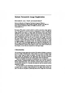
We note first that the proposed smoother given by (26) shows the interaction between the actual fixed point iteration that overcomes the nonlinearity of the operator Nl at each outer step ν and the ω-PCGS method that solves the resulting linear system of equations at each corresponding inner step k. Second, instead of solving the linear system of equations using the inner solver (28) with very high precision, it can perform only a few iteration to obtain an approximation solution at each outer step. Evidently, this procedure leads to a slight difference of convergence in the fixed point scheme when the proposed smoother is used as a stand-alone solver, whereas the computational costs significantly reduce; see Fig. 1(a). Moreover, the relaxation parameter ω also has a strong influence on the convergence speed. As the stand-alone solver of (26) we usually use ω > 1, typically ω = 1.85, because it results in speeding up the convergence compared with the PCGS approach (ω = 1); see Fig. 1(b). For our multigrid algorithm, however, we use the local Fourier analysis and several experiments to select the optimal value of ω; see Section 3.2 later. Finally we remark that other iterative techniques such as the line relaxation techniques or the preconditioned conjugate gradient method may also be used as an inner solver. However, the ω-PCGS relaxation method appears a cheaper option for practical applications. Implementation of our proposed smoother (26) based on the ω-PCGS method (28) on a fine grid can be summarized as follows: Algorithm 3 (Our Proposed Smoother). Denote by α regularization parameter ω relaxation parameter GSiter the maximum number of ω-PCGS iterations

[v1h , v2h ] ← Smoother (v1h , v2h , g1h , g2h , Rh , T h , α, ω, GSiter ).

662


a

b

No. of ν (outer iter.) VS. GSiter

No. of ν (outer iter.) VS. ω 1000

300

800 No. of ν (outer iter.)

No. of ν (outer iter.)

250 200 150 100

400

200

50 0

600

2

4

6 GSiter

8

10

0

1

1.2

1.4

ω

1.6

1.8

2

Fig. 1. Number of outer iterations ν in (26) used to drop the mean of relative residuals of (24) to 10−8 for different values of (a) GSiter and (b) ω at a fixed value of α = 0.1 for processing the registration problem in Examples 1 as shown in Fig. 3(a)–(b) on a 32 × 32 grid. The red diamond indicates the optimal choice in each plot.

• Use input parameters to compute (σlm [v h ])i,j , (G[v h ])i,j , and (N[v h ]i,j )−1 for l, m = 1, 2, 1 ≤ i ≤ n1 , and 1 ≤ j ≤ n2 (Here (v h )i,j = ((v1h )i,j , (v2h )i,j )⊤ ). • Perform ω-PCGS steps – for k = 1 : GSiter – for i = 1 : n1 – for j = 1 : n2 – Compute

(v h )[i,kj+1] = ((v1h )[i,kj+1] , (v2h )[i,kj+1] )⊤ using (28) – end – end – end We remark that in a different context [48,32] for a different technique, a first-order approximation of T (u[ν+1] ) = T (x + u[ν+1] ) = T (x + u[ν] + δ u[ν] ) [ν] [ν] ≈ T (x + u[ν] ) + ∂u1 T (x + u[ν] )δ u[ν] 1 + ∂u2 T (x + u )δ u2 ,

(29)

similar to expanding fl (u1 , u2 ) in (25) is used to derive the FP schemes. We also wish to remark that the above quantities σl1 (u[ν] ), σl2 (u[ν] ) may be refined to derive a cheaper implementation than our FP method (26). We note first that σ21 (u[ν] ) = σ12 (u[ν] ). Second in order to have a simple and stable numerical scheme as pointed out by several works; see e.g. [18] and [3, p. 56/79], we approximate σlm (u[ν] ) by σlm (u[ν] ) = (∂ul T (u[ν] ))(∂um T (u[ν] )) for m = 1, 2 since the image difference T (u[ν] ) − R becomes small for well registered images and the second-order derivatives of T (u[ν] ) (∂um ul T (u[ν] )), a problematic part of σlm (u[ν] ), are very sensitive to noise and are hard to estimate robustly. Finally, we note that if discrete image gradient ∂ul T (u[ν] ) does not vanish at one point, the system matrix of these linearized equations is strictly or irreducibly diagonally dominant. This guarantees the existence of a unique solution of each linearized system and global convergence of the Jacobi and GS iterations [49,50]. Below we analyze the smoothing property of our proposed smoother (26). [ν+1]

[ν+1]

3.2. Local Fourier analysis (LFA) LFA is a powerful tool to analyze the smoothing properties of iterative algorithms used in MG methods. Although LFA was originally developed for discrete linear operators with constant coefficients on infinite grids, it can also be applied to more general nonlinear equations with varying coefficients such as the discrete version of (5). To this end, first an infinite grid is assumed to eliminate the effect of boundary conditions and second it is also assumed that the discrete nonlinear operator can be linearized (by freezing coefficients) and replaced locally by a new operator with constant coefficients [30].


663

This approach has proved to be very useful in the understanding of MG methods when solving nonlinear problems; see for instance [42,51,43,44,52,12,53,54,18,55] for interesting examples and discussions. 3.2.1. Measure of h-ellipticity It is well known that h-ellipticity is crucial for multigrid methods to be effective. It is often used to decide whether or not pointwise error smoothing procedures (e.g. our proposed smoother (26) based on (28)) can be constructed for the discrete h h operator under consideration. To this end, we shall show that the linearized system Nh [u ]uh = Gh [u ] in (26) at some outer step provides a sufficient amount of h-ellipticity in a similar way shown in [12,18,30,40] for a discrete system of PDEs. Here h h h uh and u denote the exact solution and the current approximation and Nh [u ] and Gh [u ] the resulting discrete operators h from the linearization at u . For simplicity, our analysis is carried out over the infinite grid

Ωh∞ = {x ∈ Ω |x = (x1i , x2j )⊤ = ((2i − 1)h/2, (2j − 1)h/2)⊤ , i, j ∈ Z2 }

(30)

where h = 1/n denotes the mesh parameter. Let ϕh (θ, x) = exp(iθx/h) ·  I be grid functions, where  I = (1, 1)⊤ , θ = (θ1 , θ2 )⊤ ∈ 2 = (−π , π]2 , x ∈ Ωh∞ , and √ i = −1. It is important to remark that due to the locality nature of LFA, our analysis applies to each grid point separately, i.e. we consider the local discrete system Nh (ξ )uh = Gh (ξ ) centered and defined only within a small neighborhood of each grid point ξ = (i, j) and uh (ξ ) = [uh1 (ξ ), uh2 (ξ )]. Applying the discrete operator Nh (ξ ) to the grid functions ϕh (θ, x), i.e. Nh (ξ )ϕh (θ, x) =  Nh (ξ , θ)ϕh (θ, x), yields the Fourier symbol as follows:

[ h (θ) + σ11 (ξ ) −α L  Nh (ξ , θ) = σ21 (ξ )

] σ12 (ξ ) h (θ) + σ22 (ξ ) −α L

(31)

h (θ) denotes the Fourier symbol of the discrete (see details related to Fourier symbols of systems of PDEs in [30,40]). Here L h  Laplacian operator L . Following [30,40], the measure of h-ellipticity is defined via  Nh (ξ, θ) as follows: Eh (Nh (ξ )) =

min{| det( Nh (ξ , θ))| : θ ∈ Θhigh } max{| det( Nh (ξ , θ))| : θ ∈ 2}

,

(32)

where 2high = 2 \ (−π /2, π /2]2 denotes the range of high frequencies and

h (θ))2 + α c1 (L h (θ)) + c2 det( Nh (ξ , θ)) = α 2 (L

(33)

represents the determinant of  Nh (ξ , θ) where c1 = −(σ11 (ξ ) + σ22 (ξ )) and

c2 = σ11 (ξ )σ22 (ξ ) − σ12 (ξ )σ21 (ξ ).

For the Laplacian, we have

h (θ) = (2/h2 )(2 − (cos θ1 + cos θ2 )), −L

h (θ)) = −L h (−π /2, 0) = 2/h2 min (−L

θ∈2high

h (θ)) = −L h (π , π ) = 8/h2 . Therefore, and maxθ∈2 (−L Eh (Nh (ξ )) =

2α + c1 h2 + (c2 h4 /2α) 32α + 4c1 h2 + (c2 h4 /2α)

(34)

and lim Eh (Nh (ξ )) =

h→0

1 16

(35)

bounded away from 0 for all possible choices α, h > 0 and for all possible values of σ11 (ξ ), σ12 (ξ ), σ21 (ξ ), and σ22 (ξ ) (i.e. the results do not depend on the given images) over the whole discrete domain Ωh . h h As a result, the discrete system Nh [u ]uh = Gh [u ] is appropriate to pointwise error smoothing procedures and so is our proposed smoother (26) combined with the ω-PCGS method (28). 3.2.2. Smoothing analysis for the proposed smoother A robust and potential smoother has to take care of the high-frequency components of the error between the exact solution and the current approximation since the low-frequency components becomes the high-frequency components on coarser grids and they cannot be reduced on coarser grids by the coarse-grid correction procedure. A quantitative measure of the smoothing efficiency for a given algorithm is the smoothing factor denoted by µ from a LFA and numerically computed for test problems, which is defined as the worst asymptotic error reduction, by performing one smoother step, of all highfrequency error components [30,40]. Below we shall analyze the smoothing properties of the proposed smoother via (26) and (28).

664


As pointed out in many cases of nonlinear operators with varying coefficients in [42,51,43,44,52,12,53,54,18,55], the smoothing factor is x-dependent. Therefore, it is customary to look for the maximum over the local smoothing factors of the frozen operator Nh (ξ ), i.e.

µ∗loc = max µloc .

(36)

ζ ∈Ωh

To determine µloc we consider again the local discrete system Nh (ξ )uh (ξ ) = Gh (ξ ). By using the splitting Nh (ξ ) = [+] [0] [−] Nh (ξ ) + Nh (ξ ) + Nh (ξ ), it is possible to write the local inner iterations of (26) (for ω = 1) as Nh (ξ )unew (ξ ) + Nh (ξ )unew (ξ ) + Nh (ξ )uold (ξ ) = Gh (ξ ) [+]

where and

h uold

[0]

h

(ξ ) and

[+/0/−]

Nh

h unew

 (ξ ) =

[−]

h

h

(37)

(ξ ) stand for the approximations to uh (ξ ) before and after the inner smoothing step, respectively [+/0/−]

(ξ ))1,1

(Nh

[+/0/−]

(ξ ))2,1

(Nh

(Nh (Nh

[+/0/−]

(ξ ))1,2

[+/0/−]

(ξ ))2,2

 .

For a specification of this splitting, we use the stencil notation as follows: h

L[+] = [+/−]

(Nh

α h2

0 −1 0

0 0 −1



(ξ ))l,m =



0 0 , 0



Lh[+/−]

Lh[0]

=

for l = m for l ̸= m,

0,

α

0 0 0



h2

0 1 0

0 0 , 0



h

L[−] =

α h2

0 0 0



−1 0 0

0 −1 , 0



(N[h0] (ξ ))l,m = κl,m Lh0 (l, m = 1, 2),

and

κ=

[ κ1,1 κ2,1

] [ κ1,2 Σ + (h2 /α)σ11 (ξ ) = κ2,2 (h2 /α)σ21 (ξ )

] (h2 /α)σ12 (ξ ) . Σ + (h2 /α)σ22 (ξ )

By subtracting (37) from Nh (ξ )uh (ξ ) = Gh (ξ ) and defining enew (ξ ) = uh (ξ ) − uhnew (ξ ) and eold (ξ ) = uh (ξ ) − uhold (ξ ) we obtain the local system of error equations h

h

Nh (ξ )enew (ξ ) + Nh (ξ )enew (ξ ) + Nh (ξ )eold (ξ ) = 0 [+]

[0]

h

[−]

h

h

or enew (ξ ) = −[Nh (ξ ) + Nh (ξ )]−1 [Nh (ξ )]eold (ξ ) = Sh (ξ )eold (ξ ) h

[0]

[+]

[−]

h

h

(38)

where Sh (ξ ) is the amplification factor. The effect of Sh (ξ ) on the grid functions ϕh (θ, x) within 2high = 2 \ [−π /2, π /2]2 will determine the smoothing properties of the PCGS method (27). For the ω-PCGS approach (28), the amplification factor denoted by Sh (ξ , ω) can be defined in a similar way as (38) and its Fourier symbol is given by

 Sh (ξ , θ, ω) = [ N0 (ξ , θ) + ω N+ (ξ , θ)]−1 [(1 − ω) N0 (ξ , θ) − ω N− (ξ , θ)] ∈ C2×2 . h

h

h

h

(39)

[+/0/−]

(ξ ) are [ [+/0/−] ] [+/0/−] ( Nh (ξ , θ))1,1 ( Nh (ξ , θ))1,2 [+/0/−]  . Nh (ξ , θ) = [+/0/−] [+/0/−] (ξ , θ))2,1 ( Nh (ξ , θ))2,2 (Nh

Here the Fourier symbols of Nh

(40)

Therefore, the local smoothing factor is

µloc = sup{|ρ( Sh (ξ , θ, ω))| : θ ∈ 2high } where ρ indicates the spectral radius of  Sh (ξ , θ, ω). Recall that  α − 2 (exp(−iθ1 ) + exp(−iθ2 )) for l = m (N[+] h h (ξ , θ))l,m = 0, for l ̸= m,  α − 2 (exp(iθ1 ) + exp(iθ2 )) for l = m (N[−] h h (ξ , θ))l,m = 0, for l ̸= m α (N[h0] (ξ , θ))l,m = 2 κl,m

(41)

(42)

(43)

(44) h will be used to compute (39). To select the optimal value of ω and test our smoother we consider one set of medical images as shown respectively in Fig. 3(a)–(b) on a 32 × 32 grid. Fig. 2 shows the smoothing factors of the proposed smoother (26) based on the ω-PCGS approach (28) at different values of ω. It indicates that the optimal value ω providing µ∗loc ≈ 0.5 is not exactly 1 but very close to 1, typically ω = 0.9725.


665

μ*locVS. ω 1 0.9

μ*loc

0.8 0.7 0.6 0.5 0.4

0

0.5

1 ω

1.5

2

Fig. 2. Smoothing factors µ∗loc at a fixed value of α = 0.1 after 5 outer iterations with GSiter = 5 by the proposed smoother (26) based on the ω-PCGS approach (28) with different values of ω for the registration problem in Examples 1 as shown in Fig. 3(a)–(b) on a 32 × 32 grid. The red diamond indicates the optimal value of ω.

3.3. A nonlinear multigrid algorithm with automatic selection of α As is typical of Tikhonov regularization, the energy functional Jα in (2) has a regularization parameter α . To provide well matched images, we have to carefully select α because it is in general unknown a priori. In order to find a suitable α automatically, we follow the ‘cooling’ (‘continuation’) process suggested in [56–58,12,15,59,60]. The basic idea is to start with a high initial value of α and then slowly reduce α such that the obtained solution can be used to be an excellent starting point for the next in order to decrease Jα . An alternative approach can be the L-curve method. Consider the discrete version of the minimization problem (2) with the same notation min Jα [u] = D (R, T (u)) + α R(u).

(45) (s+1)

(s)

Let α1 be the initial value, which is sufficiently large. At the (s + 1)th step we set α = βα ∈ [α0 , α1 ], where β ∈ (0, 1) is a constant, usually chosen to be about 0.5, and α0 is a small positive number, e.g. 5 × 10−5 . Subsequently, we apply α (s+1) (s+1) and the initial guess solution obtained by the previous iteration uinitial = u(s) with the associated inner loop to obtain the minimum u(s+1) within some tolerance. As mentioned in [58], since the functional Jα is changing at each outer loop iteration, the demand of decreasing the value of the same functional is not reasonable. Then, the solution u(s+1) and parameter α (s+1) are acceptable if they satisfy the so-called consistent condition:

Jα (s+1) [u(s+1) ] = D [u(s+1) ] + α (s+1) R[u(s+1) ] < Jα (s+1) [u(s) ] = D [u(s) ] + α (s+1) R[u(s) ]. However, if this condition is not satisfied, we increase β (usually to 0.9) and re-start the step. Our experience suggests that the stopping criterion given by

‖u(s+1) − u(s) ‖l2 0 is small (normally set to 10−3 ). Finally, we summarize this process as follows: Algorithm 4 (Multigrid Image Registration Through Cooling).

→ [v ∗ , α ∗ ] ← cooling (v (0) , α (0) , − ε ). • Set s = 1, v (s) = v (0) , α (s) = α (0) , β = 0.5. • Outer iteration: For s = 1, 2, 3, . . . – 1. Set α (s+1) = βα (s) in [5 × 10−5 , α (s) ]. − → – 2. Inner iteration: vnew ← FASMG(v (s) , α (s+1) , ε ). (s) – 3. If Jα (s+1) [vnew ] < Jα (s+1) [v ]. – 3.1 Set v (s+1) = vnew , β = 0.5, s = s + 1, and go to 4. Else – 3.2 Set β = 0.9, and go to 4. – 4. Check for convergence using the criterion (46). If not satisfied, then return to 1, else, exit to the next step to stop. • Set v ∗ = vnew and α ∗ = α (s) .

(46)

666


− →

In order to save computational work for high-resolution digital images, the low-tolerance ε lo = (2, 10−4 , 0.1, 10−4 ) is applied to reduce the accumulated costs in each minimization problem. Then our first algorithm, namely a robust diffusion image registration (RDR) approach, can be stated as follows: Algorithm 5 (The Basic RDR Method).

− →

1. Input ε lo .Set α = 1 (optional). Set − → ε hi = (20, 10−8 , 0.10, 10−8 ) (high-tolerance). 2. Obtain the optimal regularization parameter α (through cooling) via Algorithm 4: − → – [v (0) , α] ← cooling (v , α, ε lo ). 3. Solve the discrete minimization problem (45) on the finest level using the found α : − → – v ← FASMG(v (0) , α, ε hi ). Although the above algorithm enables us to find a good α , the cost of resolving the same problem repeatedly is expensive. We propose to use a hierarchy of L grids (with level L the finest and level 1 the coarsest one) using a multi-resolution idea to gain efficiency while finding an effective α . Firstly we shall seek the optimal α on the coarsest level 1 with the grid size of 32 × 32 only (believed to be coarse enough) and secondly we use the multilevel continuation idea [12] to provide the initial guesses for the next finer level. Algorithm 6 (Multilevel Grid Continuation for Optimal α and Reliable Initial Solution).

[v

[lev]

, α [lev] ] ← RDR_multiresolution(v

[lev]

→ , α [lev] , lev, − ε ).

• If lev = 1

– v [lev] = 0 –α [lev] = C [C > 0 should be large enough e.g. C = 100] − → – [v [lev] , α [lev] ] ← cooling (v [lev] , α [lev] , ε ) • Else [lev] [lev] – v [lev−1] = (IhH v1 , IhH v2 )⊤ [lev−1] [lev−1] – [v ,α ]← − → RDR_multiresolution(v [lev−1] , α [lev−1] , lev − 1, ε ) h [lev−1] h [lev−1] ⊤ [lev] ) , IH v 2 –v = ( IH v 1 –α [lev] = 4α [lev−1] [Recall that α [lev] = α n2lev and nlel = 2nlel−1 ] − → – v [lev] ← FASMG(v [lev] , α [lev] , ε ) • Endif Finally the overall procedure of finding an optimal α and then starting a nonlinear multigrid method to solve (2) is summarized below as Algorithm 7: Algorithm 7 (The Refined RDR Multi-Resolution Method).

− →

− →

1. Input ε lo and ε hi . 2. Obtain the optimal regularization parameter α (through cooling) and a good initial solution (through multi-resolution) v(0) via Algorithm 6: − → – [v (0) , α] ← RDR_multiresolution(v [L] , α [L] , L, ε lo ). 3. Solve the minimization problem (45) on the finest level lev = L using the found α and the initial guess solution v (0) : − → – v [lev] ← FASMG(v (0) , α, ε hi ).


667

4. An application of Algorithm 7 to a curvature model To test the robustness of our numerical algorithm for other registration models, in this section, we shall examine our second test model, namely, the curvature image registration model, as introduced in [5,6]; see also [7,18,33,3]. The curvature model. Based on an approximation of the mean curvature of the surface of ul , Fischer–Modersitzki’s curvature approach aims to find a reasonable deformation field u that minimizes the following functional [5,6]

Jα (u) = D (u) + α RCv (u) where RCv is as in (4). This leads to the Euler–Lagrange system of two fourth-order nonlinear PDEs:



f1 (u) + α ∆2 u1 = 0 f2 (u) + α ∆2 u2 = 0

(Fischer–Modersitzki’s curvature model)

(47)

subject to the special boundary conditions ∇ ul = 0, ∇ 1ul = 0 on ∂ Ω , for l = 1, 2. We remark that the use of second-order derivatives in the energy functional (4) not only provides smoother deformation fields u than those of (3), but also allows for an automatic rigid alignment. Here ul is understood as a surface in R3 represented by (x1 , x2 , ul (x1 , x2 )), where initially ul (x1 , x2 ) = 0, with the mean curvature of the surface of ul is given by

κM (ul ) = ∇ · 

∇ ul

=

(1 + u2lx )ulx 1

1 + |∇ ul |2

1 x1

− 2ulx ulx ulx 1

2

1 x2

+ (1 + u2lx )ulx 2

(1 + u2lx + u2lx )3/2 1

2 x2

.

(48)

2

Observe that |∇ ul | ≈ 0 yields κM (ul ) ≈  κM (ul ) = 1ul . See also [24]. Since the biharmonic operator which appears in (47) is known to lead to poor multigrid efficiency, therefore, it is common to split up the equation into a system of two Poisson-type equations; see [37,38,16,18,30,39,40]. Based on this splitting idea, (47) can be converted to the following system using additional unknown functions v1 = −1u1 and v2 = −1u2 :

 −1u1 − v1 = 0   −1u2 − v2 = 0  f1 (u) − α 1v1 = 0 f2 (u) − α 1v2 = 0

(49)

subject to the boundary conditions transferred into ∇ ul = 0 and ∇vl = 0 on ∂ Ω where the data term fl (u) is given by (5). To solve the above continuous system numerically, (49) is first discretized by the cell-centered finite difference scheme over the discrete domain

Ωh = {x ∈ Ω |x = (x1i , x2j )⊤ = ((2i − 1)h/2, (2j − 1)h/2), 1 ≤ i, j ≤ n} consisting of N = n2 cells of size h × h with grid spacing h = 1/n. Let (zh )i,j = zh (x1i , x2j ) denote the grid function for l l l = 1, . . . , 4, where z h = uh or v h for l = 1, 2. Then, the discrete system of (49) at a grid point (i, j) is given by  l l l

−Lh (uh ) − (v h ) = (g h ) 1 i ,j 1 i ,j 1 i,j        h h  N1 (z )i,j     h  −L (uh2 )i,j − (v2h )i,j = (g2h )i,j        h h N2 (z )i,j

(50)

 ( , uh2 )i,j − α Lh (v1h )i,j = (g3h )i,j          N3h (z h )i,j      f h (uh , uh ) − α Lh (v2h )i,j = (g4h )i,j ,   2 1 2 i,j   f1h

uh1

N4h (z h )i,j

l = 1, . . . , 4) on the finest where (z h )i,j = ((z1h )i,j , (z2h )i,j , (z3h )i,j , (z4h )i,j )⊤ = ((uh1 )i,j , (uh2 )i,j , (v1h )i,j , (v2h )i,j )⊤ and (gh )i,j = 0 ( l

grid in multigrid setting. Recall that the discrete versions of Lh and flh (uh1 , uh2 )i,j are given in the same way as represented by Section 2.2 and the approximations used in (50) need to be modified at grid points near the image boundary ∂ Ωh using the homogeneous Neumann boundary conditions approximated by one-side differences for boundary derivatives:

(zlh )i,1 = (zlh )i,2 ,

(zlh )i,n = (zlh )i,n−1 ,

(zlh )1,j = (zlh )2,j ,

(zlh )n,j = (zlh )n−1,j .

(51)

A robust smoother based on the linearization scheme (25). As mentioned above, our aim is to apply our linearization idea (25) in solving the equivalent system (49). This leads to the linearized system NCv [z [ν] ]z [ν+1] = GCv [z [ν] ],

(52)

668


where the symbols h and (·)i,j in (50) are dropped for simplicity. Here

−L



 0 NCv [z [ν] ] =  σ11 (u[ν] ) σ21 (u[ν] )

0

−1

−L σ12 (u[ν] ) σ22 (u[ν] )

−α L

0 0

0 −1  0 

 (53)

−α L

and





g1   g2  GCv [z [ν] ] =  [ν] [ν] [ν] [ν] [ν]  . g3 − f1 (u[ν] , u ) + σ ( u ) u + σ ( u ) u 11 12 1 2 1 2 [ν] [ν] [ν] [ν] g4 − f2 (u1 , u2 ) + σ21 (u[ν] )u1 + σ22 (u[ν] )u2

(54)

As mentioned in Section 3.1, σ21 = σ12 and σlm = (∂ul T (u[ν] ))(∂um T (u[ν] )) for m = 1, 2 are used to stabilize our numerical scheme. In order to solve (52), we again apply the ω-PCGS as the inner solver and its kth step is updated by [ν]

[ν]

[ν]

[k+1/2]

(z [ν+1] )i[,kj+1] = (1 − ω)(z [ν+1] )[i,kj] + ω(NCv [z [ν] ]i,j )−1 (GCv [z [ν] ])i,j

(55)

where



(Σ )i,j /h2

 0 NCv [z [ν] ]i,j =  (σ11 (u[ν] ))i,j

(σ21 (u ))i,j [ν]

0

−1

(Σ )i,j /h2 (σ12 (u[ν] ))i,j (σ22 (u[ν] ))i,j

α(Σ )i,j /h2

0 0



0 −1 0

α(Σ )i,j /h

2

  

2 at (1, 1), (n, 1), (n, 1), and (n, n) (four corners) (Σ )i,j = 3 for all (1, j), (n, j), (i, 1), and (i, n) where 2 ≤ i, j ≤ n − 1 (boundary lines) 4 for all (i, j) where 2 ≤ i, j ≤ n − 2 (interior points),   [k+1/2] (g1 )i,j + (1/h2 )(Σ )i,j (u1[ν+1] )i,j   [k+1/2] (g2 )i,j + (1/h2 )(Σ )i,j (u2[ν+1] )i,j     [ν] [ν] [ν]   [ν] (g3 )i,j − f1 (u1 , u2 )i,j + (σ11 (u ))i,j (u1 )i,j   Cv [ν] [k+1/2] (G [z ])i,j = ,  + (σ12 (u[ν] ))i,j (u[ν] )i,j + (α/h2 )(Σ )i,j (v [ν+1] )[k+1/2]  i ,j 1 2     [ν] [ν] [ν]   (g4 )i,j − f2 (u[ν] 1 , u2 )i,j + (σ22 (u ))i,j (u2 )i,j

(56)



(57)

(58)

[k+1/2]

[ν+1] 2 + (σ21 (u[ν] ))i,j (u[ν] )i,j 1 )i,j + (α/h )(Σ )i,j (v2

and [k+1/2]

(Σ )i,j (zl[ν+1] )i,j

1] = (zl[ν+1] )[i+k]1,j + (zl[ν+1] )[i−k+1,1j] + (zl[ν+1] )i[,kj]+1 + (zl[ν+1] )[i,kj+ −1 .

(59)

With the above smoother, the curvature model can be solved using our Algorithms 7–7. 1 Similarly to Section 3.2, we can show by the LFA that (1) limh→0 Eh (NCv h (ξ )) = 256 , i.e. the linearized system (52) is helliptic; and (2) ω ≈ 1 (typically ω = 0.9725) provides the good smoothing properties (µ∗loc ≈ 0.5), where the effects of ω on smoothing factors of (55) in processing the registration problem shown in Fig. 3(a)–(b) are almost identical with Fig. 2. We also conducted several numerical tests to confirm that (52) is a robust smoother for the FAS-NMG method to solve the curvature model (47); see Section 5.2. 5. Numerical experiments The main aim of this section is to show that our new Algorithm 7 using (25) is effective and robust in leading to convergent multigrid methods in the FAS-NMG framework for both the diffusion and curvature models. In all experiments, the bilinear interpolation was used to compute the transformed template image T (u). 5.1. The diffusion model tests We first focus on the performance of Algorithm 7 for two sets of medical data, Examples1 1 and 2 shown respectively in Fig. 3(a)–(b) and (d)–(e). We first consider its convergence behavior with different resolutions, and then show comparisons with several other methods. In all experiments for this section ν1 = 5, ν2 = 5, GSiter = 5, and ω = 0.9725 were used in this test. 1 Source: http://www.math.mu-luebeck.de/safir/.


a

b

c

d

e

f

669

Fig. 3. Registration results for X-ray and MRI images using the RDR method with Algorithms 2, 5, and 7. Left column: reference R, center column: template T , right column: the deformed template image T (u) obtained from Algorithm 7. Table 1 Registration results of Algorithms 2, 5, and 7 for Examples 1 and 2 shown in Fig. 3(a)–(b) and (d)–(e). The letters ‘M’, ‘R’, ‘D’, ‘C’, and ‘IC’ mean the number of multigrid steps, the relative reduction of residual, the relative reduction of dissimilarity, the total runtimes, and the initial runtimes for determining the optimal α and initial guess u(0) , respectively. Algorithm 2 M/R/D/C

Algorithm 5 M/R/D/IC/C

Algorithm 7 M/R/D/IC/C

Example 1: h = 1/128 h = 1/256 h = 1/512 h = 1/1024

α = 0.1000 10/2.1 × 10−9 /0.1082/4.3 11/3.6 × 10−9 /0.1161/22.5 11/2.8 × 10−9 /0.1221/106.4 11/8.6 × 10−9 /0.1239/472.6

6/1.8 × 10−9 /0.1082/7.9/10.1 6/3.1 × 10−9 /0.1161/41.2/54.2 6/2.5 × 10−9 /0.1221/180.1/231.9 6/3.8 × 10−9 /0.1239/798.1/1049.3

7/3.4 × 10−9 /0.1082/2.1/6.2 7/5.1 × 10−9 /0.1161/3.9/24.2 6/7.5 × 10−9 /0.1221/7.3/65.1 6/8.2 × 10−9 /0.1239/26.1/256.4

Example 2: h = 1/128 h = 1/256 h = 1/512 h = 1/1024

α = 0.1176 10/8.3 × 10−9 /0.0522/4.2 11/5.6 × 10−9 /0.0582/22.9 11/7.4 × 10−9 /0.0615/108.3 11/3.1 × 10−9 /0.0633/478.1

5/1.5 × 10−9 /0.0522/7.2/10.2 6/2.6 × 10−9 /0.0582/31.3/41.7 7/5.4 × 10−9 /0.0615/185.7/234.9 7/6.9 × 10−9 /0.0633/550.1/943.1

6/4.2 × 10−9 /0.0552/2.9/4.9 7/6.9 × 10−9 /0.0582/3.0/17.9 7/3.3 × 10−9 /0.0615/12.5/79.1 7/5.0 × 10−9 /0.0633/26.9/321.3

5.1.1. h-independent convergence tests One of the key properties of multigrid techniques is that their convergence does not depend on the number of grid points. Thus, in the first test we designed our experiments to investigate this property with Algorithms 2, 5, and 7, and to back up our theoretical results by LFA in Section 3.2. The number of multigrid steps (V-cycles) used to drop the mean of the relative residual below ε2 = 10−8 , the relative reduction of dissimilarity, and runtimes (in seconds) are given in Table 1 with different sizes of grid points. The results show that all registration algorithms not only converge within a few multigrid steps, but they are also accurate because the dissimilarities between the reference and registered images have been reduced more than 87% for Example 1 and 94% for Example 2. For overall performance the experimental results suggest that Algorithm 7 would be preferred for practical applications because the multi-resolution idea used in the cooling process for α has been prove to be very useful for initialization. 5.1.2. Comparison with other multigrid methods Methods in [4,12,18,21,22] are some existing unilevel or multigrid techniques used to solve the diffusion model.

670

N. Chumchob, K. Chen / Journal of Computational and Applied Mathematics 236 (2011) 653–674 Table 2 A comparison among different multigrid methods in [4,12,18,21,22] to solve the diffusion model in the first 20 iterations. The letters ‘M’, ‘R’, and ‘D’ mean the number of iterations in dropping the mean of the relative residuals resulting form (2) to 10−8 , the mean of the relative residuals, and the relative reduction of dissimilarity, respectively. Our proposed multigrid method in the last row is clearly the fastest in convergence. Methods

M/R/D

Multi-resolution + AOS [4] Multi-resolution + FMG-V(2, 2) [21] Multi-resolution + Gauss–Newton + LMG-V(2, 2) [12,18] FAS-NMG-V(5, 5) + MSFP-FS smoother adapted from [8,9] (Section 2.4.3) FAS-NMG-V(5, 5) + MSFP-1 smoother adapted from [22,3] (Section 2.4.3) FAS-NMG-V(5, 5) + MSFP-2 smoother adapted from [43] (Section 2.4.3) FAS-NMG-V(5,5) + RFP smoother (26) (Section 3.1)

20/7.1 × 10−4 /0.1417 20/5.9 × 10−4 /0.1428 20/6.3 × 10−7 /0.1344 20/2.6 × 10−5 /0.1377 18/4.5 × 10−9 /0.1351 18/7.6 × 10−9 /0.1383 11/2.0 × 10−9 /0.1329

Table 3 Registration results of Algorithm 2 and AOS method [5] for Example 1 shown in Fig. 3(a)–(b). ∗ indicates either computation stopped after about 24 h or failure in dropping the relative residual to 10−8 in 10,000 iterations. Note that a much smaller residual tolerance of 10−1 is practically needed; here we test for convergence.

h h h h

= 1/128 = 1/256 = 1/512 = 1/1024

Algorithm 2 M/R/D/C

AOS M/R/D/C

10/8.6 × 10−9 /0.1248/4.2 (0.07 min) 11/2.0 × 10−9 /0.1329/23.1 (0.38 min) 11/9.4 × 10−9 /0.1383/105.2 (1.75 min) 11/4.7 × 10−9 /0.1404/427.6 (7.96 min)

10000/ ∗ /0.1248/934.1 (>15 min) 10000/ ∗ /0.1329/5500.8 (>1.5 h) 10000/ ∗ /0.1383/2498.3 (>6.9 h) ∗/ ∗ / ∗ /∗ (>24 h)

In this section, we took Examples 1 to illustrate a comparison among our FAS-NMG method with Algorithm 2 and other six multigrid methods by starting with the fixed parameters h = 1/256, α = 1/8 and u(0) = 0. Here we used τ = 10−2 and applied the so-called multi-resolution technique with the gradient descent methods of [4,21] for fairness. The FMG or LMG methods in [12,18,21] were performed using two pre-smoothing and two post-smoothing steps with the pointwise GS smoothers until the mean of relative residuals below a user-supplied threshold (tolLMG = 10−4 ). Table 2 summarizes the results for all multigrid methods. As expected from the experiments, all methods are very fast and accurate in registering the given images because the dissimilarities between the reference and registered images have been reduced more than 80% within the first 20 iterations. However our method is not only the fastest way in solving the problem, but also in dropping the mean of the relative residuals below 10−8 . 5.1.3. Comparison with the AOS method [4] The AOS method is one of the most widely used gradient descent techniques for diffusion image registration [4,19,21]. We take Example 1 to illustrate a comparison with our FAS-NMG method. Table 3 summarizes the results for Algorithm 2 and AOS methods with different numbers of grid points. We used Algorithm 2 with α = 1/8 for fairness (as Algorithm 7 will be even better). That is, we started both methods with the same α and the same initial guess, u(0) = 0. For the AOS method, the time-step τ is required to be sufficiently small for each size of the problem. We used τ = 10−2 for h = 1/128 − 1/1024. As expected from the experiments, both methods are very accurate in registering the given images because the dissimilarities between the reference and registered images have been reduced more than 85%. However the AOS fails to drop the relative residual to 10−8 in a few time steps (even for τ > 10−2 ) and the runtimes used by the RDR method is much faster than those of the AOS technique in delivering the same level of the relative dissimilarity. 5.1.4. Comparison of multigrid methods with different smoothers Our aim in this section is to show that we have proposed a robust smoother for the FAS-NMG technique in solving the discrete system represented in (14). To end this, we have conducted several experiments of our FAS multigrid with different kinds of smoothers: (i) the proposed smoother based on the RFP method (26) represented by Algorithm 3 in Section 3 (ii) the GS smoother based on the SFP method given by (19) in Section 2.4.3 (the standard FP method defined in [3, p. 79] with the standard linear (inner) solver) (iii) the GS smoother based on the MSFP-FS method given by (20) and (21) in Section 2.4.3 (a modified SFP method adapted from the numerical techniques of Frohn-Schauf et al. [8,9] with the standard linear solver) (iv) the GS smoother based on MSFP-1 method given by (22) in Section 2.4.3 (a modified SFP method of the first type with the standard linear solver) (v) the GS smoother based on MSFP-2 method given by (23) in Section 2.4.3 (a modified SFP method of the second type with the standard linear solver)


a

b

671

c

Fig. 4. Results from Example 1 as shown in (a)–(b) by the curvature model (47) using the FAS-NMG method with the smoother (52). Left to right: the reference R, the template T , and the registered image T (u) by the curvature model (47).

(vi) line relaxation smoothers based on the RFP method in Section 3 (the RFP method given by (26) with another kind of iterative linear solvers) (vii) the Newton–Gauss–Seidel smoother used in [10] and given explicitly in [20] in (13) (an alternative way of choice of smoothers used in solving the discrete Euler–Lagrange equations represented by (14)). Omitting the computational results, we remark that these observations can be made: (a) The smoother in (ii) requires more multigrid cycles than the proposed smoother and may not lead to the convergence of the FAS-NMG technique for small values of α . (b) As expected, the results based on the smoother (iii) do not find a solution that is the necessary condition of the original variational problem (2), although the underlying MG performs better than with other smoothers (slightly less well than with our RFP smoother). (c) The smoother in (iv)–(v) may take many multigrid cycles, not leading to the convergence of the FAS-NMG technique when the fixed point parameters c1 , c2 (or c), and ϵ are not well selected (i.e. the NMG becomes sensitive to these parameters). (d) As expected, line relaxation smoothers require less multigrid cycles but more computational costs than the proposed smoother. (e) The Newton–Gauss–Seidel smoother provide well matched images within a few multigrid steps, but it may require more multigrid cycles than the proposed smoother in leading to the convergence of the FAS-NMG technique. 5.2. The curvature model In this section, we aim to show that the FAS-NMG method with the smoother (52) based on our linearization idea (25) is effective and robust to solve the curvature model (47) within the multigrid framework similar to Algorithm 1. To this end, we took only one data set of medical images, Examples 1, as shown in Fig. 3(a)–(b). We first investigate the convergence behavior and the registration accuracy of our FAS-NMG method with different sizes of image resolutions. Second we compare three numerical solution methods for solving the curvature model (47). In all experiments, Ω = [0, 1]2 , V = [0, 1], ν1 = 10, ν2 = 10, PCGSiter = 10, and ω = 0.9725 were used. 5.2.1. h-independent convergence tests In this test, we started the registration processes with α = 10−4 , u(0) = 0, and h = 1/128, . . . , h = 1/1024. The registered image is shown in Fig. 4(c). As expected from our LFA results, Fig. 5(a)–(b) shows that our FAS-NMG approach is h-independent. It takes only a few MG steps (almost the same number) to drop the mean of the relative residuals below 10−8 . Moreover, as shown in Fig. 5(b) only one MG step can reduce the dissimilarities between the reference and the registered image more than 90% for the given registration problem. 5.2.2. Comparison with two other methods In this section we aim to investigate the performance of the FAS-NMG method with the smoother (52) and those of other two methods: the FP method (52) (the smoother used as a stand-alone solver) and the DCT-based method in [6]. We note that the FT-based method in [33,34] is faster than the DCT-based method with the ratio of 2.3 for solving each linear time-dependent problem resulting from (47). Thus, for this class of gradient descent techniques it is enough to use only the DCT-based method, which is one of the most widely used techniques for the curvature model.

672


Mean of relative residuals (MRR)

10

10

10

b

MRR VS. MG steps

0

10

–2

RSSD VS. MG steps

1

128x128 256x256 512x512 1024x1024

128x128 256x256 512x512 1024x1024

0.8 Relative SSD (RSSD)

a

–4

–6

0.6

0.4

0.2 –8

10

0

2

4 MG steps

6

0 0

8

2

4 MG steps

6

8

Fig. 5. Results from Example 1 as shown by Fig. 3(a)–(b) by the curvature model (47) using the FAS-NMG method with the smoother (52). Left to right: the histories of the mean of relative residuals (MRR) with respect to the MG steps and the histories of the relative SSD (RSSD) with respect to the MG steps.

a

RSSD VS. No. Iterations

1

FAS– NMG FP DCT

0.8

–2

10

Relative SSD (RSSD)

Mean of relative residuals (MRR)

b

MRR VS. No. Iterations

0

10

–4

10

10

–6

FAS–NMG FP DCT

0.6

0.4

0.2

–8

10

0

50 100 150 Number of Iterations

200

0 0

50 100 150 Number of Iterations

200

Fig. 6. Results from Example 1 as shown by Fig. 3(a)–(b) by the curvature model (47) using three numerical solution methods: the FAS-NMG method with the smoother (52), the FP method (52), and the DCT-based method in [6]. Left to right: (a) the histories of the mean of relative residuals (MRR) with respect to the iteration steps and (b) the histories of the relative SSD (RSSD) with respect to the iteration steps.

To this end, we started all methods with h = 1/256, α = 10−4 and u(0) = 0. For the DCT-based method, the time-step τ was selected to be τ = 10−2 (since the fixed parameters 1/h4 = N 4 = 2564 , V = [0, 1] and α = 10−4 were used in the discrete system of (47), τ = 10−2 was a reasonable time-step). Compared with the results by other two methods, Fig. 6(b) shows that our FAS-NMG method is very fast in reducing the dissimilarities between the reference and registered images. Moreover, as shown in Fig. 6(a) it takes only a few steps to drop the mean of the relative residuals (MRR) below 10−8 . This is a remarkable result to conclude that its performance in solving the curvature model (47) is much more efficient than those of the other two methods. From both tests in Sections 5.1 and 5.2 they confirm that the smoothers based on our linearization idea by (25) are effective and robust in leading to convergent multigrid methods for both the diffusion and curvature models. 6. Conclusions In this paper we first reviewed various iterative methods for solving image registration models and then addressed the problem of designing an optimal and efficient FAS-NMG technique. For the commonly used SSD model, we proposed a new, simple and yet effective fixed point smoothing scheme which is demonstrated to be more effective than a large class of other iterative methods for a diffusion model and a curvature model. A local Fourier analysis was done to confirm the effectiveness of the smoother. For an automatic way of selecting the regularization parameter α , we proposed a multi-resolution idea that seems to work well for a range of problems. Numerical results confirmed the expected robustness and excellent speed in


673

convergence compared with other competing methods. Future work will address multigrid techniques for models of multimodal deformable image registration. References [1] [2] [3] [4] [5] [6] [7] [8]

[9] [10] [11] [12] [13] [14] [15] [16] [17] [18] [19] [20] [21] [22] [23] [24] [25] [26] [27] [28] [29] [30] [31] [32] [33] [34] [35] [36] [37] [38] [39] [40] [41] [42] [43] [44] [45] [46] [47]

[48]

J. Maintz, M. Viergever, A survey of medical image registration, Med. Image Analysis 2 (1) (1998) 1–36. J. Hajnal, D. Hill, D. Hawkes, Medical Image Registration, in: The Biomedical Engineering Series, CRC Press, 2001. J. Modersitzki, Numerical Methods for Image Registration, Oxford, 2004. B. Fischer, J. Modersitzki, Fast diffusion registration, Contemporary Mathematics 313 (2002) 117–129. B. Fischer, J. Modersitzki, Curvature based image registration, Journal of Mathematical Imaging and Vision 18 (2003) 81–85. B. Fischer, J. Modersitzki, A unified approach to fast image registration and a new curvature based registration technique, Linear Algebra and its Applications 380 (2004) 107–124. B. Fischer, J. Modersitzki, Ill-posed medicine—an introduction to image registration, Inverse Problems 24 (2008) 1–19. C.F. -Schauf, S. Henn, L. Hömke, K. Witsch, Total variation based image registration, in: X.-C. Tai, K.-A. Lie, T.F. Chan, S. Osher (Eds.), Proceedings of the International Conference on PDE-Based Image Processing and Related Inverse Problems Series: Mathematics and Visualization, Springer Verlag, 2006, pp. 305–323. C.F. -Schauf, S. Henn, K. Witsch, Multigrid based total variation image registration, Comput. Visual. Sci. 11 (2008) 101–113. S. Gao, L. Zhang, H. Wang, R. de Crevoisier, D. Kuban, R. Mohan, L. Dong, A deformable image registration method to handle distended rectums in prostate cancer radiotherapy, Medical Physics 33 (9) (2006) 3304–3312. E. Haber, J. Modersitzki, Numerical solutions for volumn preserving image registration, Inverse Problems 20 (2004) 1621–1638. E. Haber, J. Modersitzki, A multilevel method for image registration, SIAM Journal of Scientific Computing 27 (5) (2006) 1594–1607. E. Haber, S. Heldmann, J. Modersitzki, Adaptive mesh refinement for non parametric image registration, SIAM Journal of Scientific Computing 30 (6) (2008) 3012–3027. S. Henn, K. Witsch, Iterative multigrid regularization techniques for image matching, SIAM Journal of Scientific Computing 23 (4) (2001) 1077–1093. S. Henn, K. Witsch, Image registration based on multiscale energy information, Multiscale Modeling and Simulation 4 (2) (2005) 584–609. S. Henn, A multigrid method for a fourth-order diffusion equation with application to image processing, SIAM Journal of Scientific Computing 27 (3) (2005) 831–849. L. Hömke, A multigrid method for anisotropic PDEs in elastic image registration, Numerical Linear Algebra with Applications 13 (2006) 215–229. H. Köstler, K. Ruhnau, R. Wienands, Multigrid solution of the optical flow system using a combined diffusion- and curvature-based regularizer, Numerical Linear Algebra with Applications 15 (2008) 201–218. J.L. -Ruiz, J.M. -Sanchez, Optimal parameters selection for non-parametric image registration methods, LNCS 4179 (2006) 564–575. W. Lu, M.L. Chen, G.H. Olivera, K.J. Ruchala, T.R. Mackie, Fast free-form deformable registration via calculus of variations, Physics in Medicine and Biology 49 (2004) 3067–3087. M. Stürmer, H. Köstler, U. Rüde, A fast full multigrid solver for applications in image processing, Numerical Linear Algebra with Applications 15 (2008) 187–200. D. Zikic, W. Wein, A. Khamene, Fast deformable registration of 3D-ultrasound data using a variational approach, LNCS 4190 (2006) 915–923. N. Chumchob, K. Chen, A variational approach for discontinuity-preserving image registration, East–West Journal of Mathematics Special volume 2010 (2010) 266–282. N. Chumchob, K. Chen, C. Brito, A fourth order variational image registration model and its fast multigrid algorithm, SIAM Journal of Multiscale Modeling and Simulation 9 (2011) 89–128. L. Rudin, S. Osher, E. Fatemi, Nonlinear total variation based noise removal algorithms, Physica D 60 (1992) 259–268. T. Chan, J. Shen, Image Processing and Analysis — Variational, PDE, Wavelet, and Stochastic Methods, SIAM Publications, Philadelphia, USA, 2005. T. Chan, K. Chen, J. Carter, Iterative methods for solving the dual formulation arising from image restoration, Electronic Transactions on Numerical Analysis 26 (2007) 299–311. K. Chen, X.-C. Tai, A nonlinear multigrid method for total variation minimization from image restoration, Journal of Scientific Computing 32 (2) (2007) 115–138. A. Brandt, Multi-level adaptive solutions to BVPs, Mathematial Computing 31 (1977) 333–390. U. Trottenberg, C. Oosterlee, A. Schuller, Multigrid, Academic Press, 2001. A. Bruhn, J. Weickert, C. Feddern, T. Kohlberger, C. Schnörr, Variational optical flow computation in real time, IEEE Transactions on Image Processing 14 (5) (2005) 608–615. A. Bruhn, J. Weickert, Multigrid platform for real-time motion computation with discontinuity-preserving variational methods, International Journal of Computer Vision 70 (3) (2006) 257–277. J. Larrey-Ruiz, R. Verdú-Monedero, J. Morales-Sánchez, A fourier domain framework for variational image registration, Journal of Mathematical Imaging and Vision 32 (2008) 57–72. R. Verdú-Monedero, J. Larrey-Ruiz, Frequency implementation of the Euler–Lagrange equations for variational image registration, IEEE Signal Processing Letters 15 (2008) 321–324. T. Lu, P. Neittaanmäki, X.-C. Tai, A parallel splitting up method and its application to Navier–Stokes equations, Applied Mathematical Letters 4 (2) (1991) 25–29. J. Weickert, B. ter Haar Romeny, M. Viergever, Effcient and reliable schemes for nonlinear diffusion filtering, IEEE Transactions on Image Processing 7 (1998) 398–410. W. Briggs, V. Henson, S. McCormick, A Multigrid Tutorial, 2nd ed., SIAM Publications, Philadelphia, USA, 2000. W. Hackbusch, Multi-Grid Methods and Applications, Springer-Verlag, Berlin, Heidelberg, New York, 1985. P. Wesseling, Multigrid Methods, Edwards, Philadelphis, PA, USA, 2004. R. Wienands, W. Joppich, Practical Fourier Analysis for Multigrid Method, Chapman & Hall/CRC, USA, 2005. K. Chen, Matrix Preconditioning Techniques and Applications, Cambridge University Press, UK, 2005. N. Badshah, K. Chen, Multigrid method for the Chan–Vese model in variational segmentation, Communications in Computational Physics 4 (2) (2008) 294–316. C. Brito-Loeza, K. Chen, Multigrid method for a modified curvature driven diffusion model for image inpainting, Journal of Computational Mathematics 26 (6) (2008) 856–875. T. Chan, K. Chen, On a nonlinear multigrid algorithm with primal relaxation for the image total variation minimization, Journal of Numerical Algorithms 41 (2006) 387–411. C.F. -Schauf, S. Henn, K. Witsch, Nonlinear multigrid methods for total variation image denoising, Comput. Visual. Science 7 (2004) 199–206. J. Savage, K. Chen, An improved and accelerated nonlinear multigrid method for total-variation denoising, International Journal of Computer Mathematics 82 (8) (2005) 1001–1015. J. Savage, K. Chen, On multigrids for solving a class of improved total variation based staircasing reduction models, in: X.-C. Tai, K.-A. Lie, T.F. Chan, S. Osher (Eds.), Proceedings of the International Conference on PDE-Based Image Processing and Related Inverse Problems Series: Mathematics and Visualization, Springer Verlag, 2006, pp. 69–94. A. Bruhn, J. Weickert, Towards Ultimate Motion Estimation: Combining Highest Accuracy with Real-Time Performance, in: Proceeding of 10th International Conference on Computer Vision ICCV 2005, vol. 1, IEEE Computer Society Press, Beijing, People’s Republic of China, 2005, pp. 749–755.

674


[49] W. Rheinboldt, Methods for Solving Systems of Nonlinear Equations, 2nd ed., SIAM Publications, Philadelphia, USA, 1998. [50] Y. Saad, Iterative Methods for Sparse Linear Systems, 2nd ed., SIAM Publications, Philadelphia, USA, 2003. [51] N. Badshah, K. Chen, On two multigrid algorithms for modelling variational multiphase image segmentation, IEEE Transactions on Image Processing 18 (5) (2009) 1097–1106. [52] T. Chan, K. Chen, An optimization-based multilevel algorithm for total variation image denoising, Multiscale Mod. Simu. 5 (2) (2006) 615–645. [53] E. Haber, R. Horesh, J. Modersitzki, Numerical optimization for constrained image registration, Numerical Linear Algebra with Applications 17 (2010) 343–359. [54] S. Hamilton, M. Benzi, E. Haber, New multigrid smoothers for the oseen problem, Numerical Linear Algebra with Applications 17 (2010) 556–576. [55] B. Seynaeve, E. Rosseel, B. Nicolaï, S. Vandewalle, Fourier mode analysis of multigrid methods for partial differential equations with random coefficients, Journal of Computational Physics 224 (2007) 132–149. [56] J. Chen, E. Haber, D. Oldenburg, Three-dimensional numerical modelling and inversion of magnetometric resistivity data, Geophysical Journal of Inter. 149 (3) (2002) 679–697. [57] N. Chumchob, K. Chen, A robust affine image registration method, International Journal of Numerical Analysis and Modeling 6 (2) (2009) 311–334. [58] E. Haber, D. Oldenburg, A GCV based method for nonlinear ill-posed problems, Computational Geosciences 4 (1) (2000) 41–63. [59] P. Lelièvre, D. Oldenburg, Magnetic forward modelling and inversion for high susceptibility, Geophysical Journal of Inter. 166 (1) (2006) 76–90. [60] G.A. Newman, G.M. Hoversten, Solution strategies for two- and three-dimensional electromagnetic inverse problems, Inverse Problems 16 (2000) 1357–1375.

A robust multigrid approach for variational image registration models

A robust multigrid approach for variational image registration models

Suggest Documents

A Variational Approach for Discontinuity-Preserving Image Registration

Interactive Multigrid Refinement for Deformable Image Registration

Interactive Multigrid Refinement for Deformable Image Registration

A Variational Approach for Color Image Segmentation

MULTIMODAL IMAGE REGISTRATION USING A VARIATIONAL ...

A FOURTH ORDER VARIATIONAL IMAGE REGISTRATION MODEL ...

MULTIMODAL IMAGE REGISTRATION USING A VARIATIONAL ...

Improved variational image registration model and a fast algorithm for ...

Robust Parametric Image Registration

A Variational Framework for Joint Image Registration, Denoising and ...

An Artificial Agent for Robust Image Registration

Multigrid Optimal Mass Transport for Image Registration and Morphing

Variational Image Registration Using Inhomogeneous Regularization

A Robust Multiresolution Registration Approach - Seeger

A generalized divergence measure for robust image registration ...

A robust similarity measure for nonrigid image registration with outliers

A Robust Similarity Measure for Volumetric Image Registration with ...

A Robust Registration Method for Real-Time Ultrasound Image Fusion

Robust Multispectral Image Registration Using ... - Semantic Scholar

Robust Image Registration Based on Mutual ...

Robust Image Registration Using Selective Correlation Coefficient

Robust image registration of biological microscopic ... - BioMedSearch

ROBUST IMAGE REGISTRATION USING LOG-POLAR ... - CiteSeerX

ROBUST RETINAL IMAGE REGISTRATION USING EXPECTATION ...