Nikolaos Nasios and Adrian G. Bors ... { nn,adrian.bors }@cs.york.ac.uk .... data and their a posteriori proba- bilities, as it is shown in the following equations: mi =.
A Variational Approach for Color Image Segmentation Nikolaos Nasios and Adrian G. Bors Department of Computer Science, University of York, York YO10 5DD, UK. { nn,adrian.bors }@cs.york.ac.uk
Abstract In this paper we use a variational Bayesian framework for color image segmentation. Each image is represented in the L*u*v color coordinate system before being segmented by the variational algorithm. The model chosen to describe the color images is a Gaussian mixture model. The parameter estimation uses variational learning by taking into account the uncertainty in parameter estimation. In the variational Bayesian approach we integrate over distributions of parameters. We propose a maximum log-likelihood initialization approach for the Variational Expectation-Maximization (VEM) algorithm and we apply it to color image segmentation. The segmentation task in our approach consists of the estimation of the distribution hyperparameters.
1 Introduction Learning a graphical model from given data can be done using Maximum Likelihood (ML) Estimation. The usual approach for the ML estimation of a mixture Gaussian distribution is the Expectation-Maximization (EM) algorithm [1, 2]. However, without a proper initialization, the EM algorithm may lead to overfitting and poor generalization. While EM provides a single solution for the parameters, Bayesian inference takes into account the uncertainty in the estimation [3, 4, 5]. We suggest a new initialization procedure for the Variational Expectation-Maximization (VEM) algorithm. Image segmentation is used as a preprocessing stage in numerous computer vision applications. EM has been applied for color image segmentation [6] together with other maximum log-likelihood approaches such as mean shift analysis [7]. In this paper we present a variational approach for color image segmentation. For finding the necessary number of Gaussian mixture components we use the Bayesian Information Criterion (BIC) [2]. Moreover, we suggest an appropriate initialization for the hyperparameters updated by the VEM algorithm [8]. The paper is or-
ganized as follows. In Section 2 we introduce a Variational Bayesian framework which is applied to the finite mixture model. A maximum log-likelihood initialization procedure is provided for the proposed algorithm in Section 3. In Section 4, we present the Variational ExpectationMaximization algorithm, while in Section 5 we describe how the algorithm can be applied in the context of color image segmentation. In Section 6, we provide some experimental results and in Section 7 we report our conclusions.
2 Variational Gaussian Mixture Models Finite mixture models provide a powerful statistical approach for modelling multivariate data. We focus our attention to Gaussian Mixture Models (GMMs) because of their excellent approximation properties. The pixel probability density function in a color image is assumed to follow that of an N -component Gaussian mixture: N X αi p p(x) = exp [D(x; µi , Σi )] (1) d |Σ | (2π) i i=1
where d is data dimension, d = 3 in the case of color space, θi = {αi , µi , Σi } represents the model parameters respectively, αi is the mixing probability, µi is the mean and Σi is the covariance matrix, while D(·) corresponds to: 1 D(x; µi , Σi ) = − (x − µi )T Σ−1 (2) i (x − µi ). 2 The distribution PN is normalized and the sum of mixing probabilities is i=1 αi = 1. In a Bayesian approach, distributions of model parameters such as the mixing probabilities, means and covariance matrices, in the case of a GMM, are described by their conjugate priors [5]. Thus, giving the normalization condition, the mixing probabilities are modelled by a joint Dirichlet distribution D(α|λ1 , · · · , λN ): P N Y Γ( N j=1 λj ) αλj −1 . (3) D(α|λ1 , · · · , λN ) ∼ QN j=1 Γ(λj ) j=1
The conjugate prior for the means is the Normal distribution N (µ|m, βS), where β is a scaling factor: N (µ|m, βS) ∼ p
1 (2π)d |βS|
exp [D(µ; m, βS)] .
(4)
The Wishart distribution W(Σ|ν, S) is the conjugate prior for the inverse covariance matrix: W(Σ|ν, S) ∼
−1 1 |S|−ν/2 |Σ|(ν−d−1)/2 e− 2 T r[S Σ] Q d ) 2νd/2 π d(d−1)/4 k=1 Γ( ν−k+1 2
(5)
where ν are the degrees of freedom, T r denotes the trace of the resulting matrix (the sum of the diagonal elements) and Γ(·) represents the Gamma function.
3 Hyperparameter Initialization In many algorithms an inappropriate initialization leads to local minimas. Variational algorithms always result in achieving a lower bound on the error, but they do not guarantee a global minimum [4]. In this paper we are proposing a hierarchical hyperparameter initialization procedure for variational training. In the first stage we apply the EM algorithm onto a subset of the given data set, considering random initializations. The resulting mean parameters are forming distributions which can be modelled by GMMs. Afterwards, a second stage EM algorithm is applied onto the distributions characterizing the mean parameters, by using the initial data samples for its initialization. The results from this dual EM process are used for initializing the hyˆ perparameters [8]. Specifically, the hypermeans m(0) are taken as the average of the resulting means from the second stage EM. The hyperparameter β is considered as a scaling ˆ and the covarifactor between the covariance matrices Σ ance matrices of the mean distributions S, calculated at the second stage EM. This hyperparameter is initialized as the ˆ −1 , which can average of the eigenvalues of the matrix ΣS be calculated as the trace of the matrix divided by the dimension of the space: PL ˆ ik S−1 ) T r(Σ ik (6) βi (0) = k=1 dL where L is the number of runs for the first stage EM algorithm. The Wishart distribution W (Σ|ν, S), that characterizes the inverse covariance matrix, is described by two hyperparameters: the degrees of freedom, which are initialized as equal to the dimensionality of the data space, ν = d, and the scale matrix S. For the initialization of S we consider ˆ resulting from the first stage EM. After the distribution of Σ applying Cholesky factorization to the covariance matrices ˆ k , we generate L d-dimensional subgaussian random vecΣ tors N from a standard Normal distribution N (0, 1). The scale matrix S is calculated as: PL Rik Nk (Nk Rik )T Si (0) = k=1 (7) L where Rk and RTk correspond to the upper and lower triangular matrices resulting from the Cholesky factorization.
The Dirichlet parameters λi are calculated using the Newton’s method as follows: ψ(λi (t)) − ψ(λi (t − 1)) (8) λi (t) = λi (t − 1) − ψ 0 (λi (t)) where t is the iteration number and ψ(λi (t)) comes from the logarithmic derivative of the Dirichlet distribution and is expressed as: N X ψ(λi,t ) = ψ( λk,(t−1) ) + E[log(ˆ αi )] (9) k=1
The second term in the iterative expression from above is the expectation of the observed sufficient statistics for the mixing probabilities αi , and is approximated by the mean of the mixing probabilities distributions. By inverting equation (9) and iterating equation (8), we can estimate the hyperparameters λi .
4 Variational Expectation-Maximization Algorithm Variational Bayes algorithm has been used for estimating hyperparameters of mixture models [5]. In our approach we use the initialization procedure described in the previous section defining the Variational Expectation-Maximization (VEM) algorithm. This algorithm is an iterative procedure which alternates between two steps: variational expectation (VE) and variational maximization (VM), [8]. In the expectation step we compute the a posteriori probabilities Pˆ (i|xj ), meaning the responsibilities of each mixture component i in generating each data sample xj , according to the following expression: � 1 1 ˆ P (i|xj ) = exp − log |Si |+ dlog 2+ 2 2 � � d N X νi + k − 1 1X ψ λk )+ + + ψ(λi ) − ψ( 2 2 k=1 � k=1 d +νi D(xj ; mi , βi Si ) − (10) 2βi where d is the number of dimensions, ψ(·) is the digamma function and D(xj ; mi , βi Si ) is given by (2). Before proceeding to the next step we perform an intermediary calculation of the mean parameters considering the a posteriori probabilities from (10): PM ˆ j=1 xj P (i|xj ) µ ˆi,V EM = PM (11) Pˆ (i|xj ) j=1
In the maximization step we update the hyperparameters characterizing distributions of parameters that maximize the log-likelihood, given the data and their a posteriori probabilities, as it is shown in the following equations: P ˆ βi (0)mi (0) + M j=1 P (i|xj ) mi = (12) PM ˆ βi (0) + P (i|xj ) j=1
Si =
M X
Pˆ (i|xj )(xj − µ ˆi,V EM )(xj − µ ˆi,V EM )T +
j=1
+Si (0) + K(ˆ µi,V EM − mi (0))(ˆ µi,V EM − mi (0))T (13)
(a) “Sunset”
where
(b) “Lighthouse”
(c) “Forest”
Figure 1. Original images. PM
M ˆ X j=1 P (i|xj ) Pˆ (i|xj ) ; βi = βi (0) + K= PM ˆ βi (0) + P (i|xj )
βi (0)
j=1
while νi = νi (0)+
M X
Pˆ (i|xj ) ; λi = λi (0)+
j=1
j=1
M X
Pˆ (i|xj ) (14)
j=1
The VEM algorithm calculates iteratively until reaching a convergence criterion, [8].
5 Color Image Segmentation An important issue in color image segmentation is the selection of an appropriate color space and that of a representative set of colors. We choose to use the L*u*v* color space for segmentation as in [6, 7]. In our case the image color space is represented by a mixture of GMM components. We employ the Bayesian Information Criterion (BIC) which corresponds to the negative of the minimum description length (MDL) criterion [2]. This criterion is expressed in terms of the data log-likelihood by adding a penalty term depending on the number of components: � � N d(d + 1) ˆ CV EM (N ) = L(θ) − 3+d+ logM (15) 2 2 ˆ is the data log-likelihood, N is the number where L(θ) of components and M that of data samples. The number of components is considered as that corresponding to the largest CV EM (N ). In order to determine the segmentation performance of the algorithm we employ the peak signalto-noise ratio (PSNR) measure between the original and the segmented images after converting them to grayscale: 255 M P SN R = 20 log10 qP (16) M 2 (x − µ ) j j=1 j
that these images have distinct properties, such as the variation in lighting in ”Sunset”, constant color areas as in ”Lighthouse” or natural textures in ”Forest” image. The data samples are obtained from the transformation of the color coordinate system from RGB to L*u*v and defines a 3-D space. The initialization was performed as described in Section 3, after applying EM onto a subspace of the data set for 10 random initializations. Then we employed the second stage EM onto the results of the first EM. After initializing the hyperparameters, we applied the VEM algorithm. The pixel classification into color regions was achieved by assigning each pixel to the region for which it has the largest a posteriori probability.
(a) N = 7
(b) N = 8
(c) N = 5
(d) N = 8
(e) N = 9
(f) N = 6
(g) N = 10
(h) N = 10
(i) N = 9
Figure 2. Segmentation results when applying the VEM algorithm: (a)-(i) Segmentation results using N Gaussian components.
where we consider a hard decision for segmenting the image in color regions based on the maximum a posteriori probability Pˆ (i|xj ) from (10). We assign the hypermean to all the pixels from the corresponding segmented region.
6 Experimental Results The proposed algorithm has been applied for segmenting several color images. We present the results for three color images, called respectively ”Sunset”, ”Lighthouse” and ”Forest”, that are shown in Figure 1. We can observe
(a) N = 7
(b) N = 8
(c) N = 5
Figure 3. Segmentation results when applying EM. Figure 2 shows the segmented images for the most appropriate number of components as indicated by the BIC criterion, plotted in Figure 4. Figure 2 shows segmented im-
ages for various numbers of mixture components and Figure 3 displays images segmented by EM. In all three color images, BIC predicted an appropriate number of mixture components. The segmentation colors in Figure 2 are given by the hypermeans as calculated by the VEM algorithm.
Method
ˆ L(θ) EM
5
2.6
PSNR (dB) ˆ L(θ)
x 10
"Forest"
2.4
2.2 Bayesian Information Criterion
Measure
VEM
2
PSNR (dB)
"Lighthouse"
1.8
1.6
Sunset (N=7) 0.3676 ± 0.005 14.76 ± 2.07 0.3759 ± 0.006 18.64 ± 0.40
Color Images Lighthouse (N=8) 0.5093 ± 0.023 12.08 ± 2.49 0.5209 ± 0.006 15.88 ± 1.08
Forest (N=5) 0.4435 ± 0.0013 5.35 ± 0.39 0.5587 ± 0.031 10.96 ± 0.59
Table 1. Comparison between EM and VEM algorithms in color image segmentation.
1.4
1.2
1
"Sunset" 3
4
5
6
7
8
9
10
Number of Components
Figure 4. Estimating the number of mixture components using BIC. In Figure 5, we display the convergence in the loglikelihood with respect to the iteration, when applying the VEM algorithm 10 times for each image. The convergence criterion that has been used is: ˆ − log(Lt−1 (θ)) ˆ log(Lt (θ)) < 0.01 (17) ˆ log(Lt (θ)) ˆ is the log-likelihood for each image at iteration t. Lt (θ) 5
2.2
x 10
References [1] A. P. Dempster, N. M. Laird and D. B. Rubin, “Maximum Likelihood from Incomplete Data via EM Algorithm,” J. of the Royal Stat. Soc., Series B , vol 39, no. 1, pp. 1-38, 1977. [2] M. Figueiredo and A. Jain, “Unsupervised learning of finite mixture models,” IEEE Transactions on Pattern Analysis and Machine Intelligence, vol. 24, no. 3, pp. 381-396, 2002.
"Lighthouse" 2
"Forest" 1.8
[3] A. Gelman, J. B. Carlin, H. S. Stern and D. B. Rubin. Bayesian Data Analysis, Chapman & Hall, 1995.
VEM log−likelihood
1.6
1.4
[4] T. Jaakkola and M. Jordan, “Bayesian parameter estimation via variational methods,” Statistics and Computing, vol. 10, pp. 25-37, 2000.
1.2
1
[5] H. Attias, “A Variational Bayesian Framework for Graphical Models,” Advances in Neural Information Processing Systems (NIPS) 12, 2000, pp. 209-215.
"Sunset" 0.8
0.6
Bayesian approach for the parameter estimation and derive the VEM algorithm as a generalization of the EM. This paper provides a solution for the VEM algorithm initialization by employing a dual EM as an intermediary stage in order to obtain initial estimates for the hyperparameters characterizing the GMM model. The experimental results provided for various color images indicated that the VEM algorithm outperforms the EM algorithm. The results obtained are promising and can be used for image compression and for image region retrieval systems based on color information.
0
2
4
6 Number of Iterations
8
10
12
Figure 5. Convergence of the log-likelihood. We compare the proposed VEM algorithm with EM algorithm using the log-likelihood and the PSNR as comparison measures. The results displayed in Table 1, show that VEM outperforms EM, and that can be also observed from the segmented images in Figures 2 and 3.
7 Conclusions We propose a new variational algorithm for color image segmentation using Gaussian mixture models. We follow a
[6] Z. H. Zhang, C. B. Chen, J. Sun, K. L. Chan, “EM algorithms for Gaussian mixtures with split-and-merge operation,” Pattern Recognition, vol. 36, no. 9, pp. 1973-1983, 2003. [7] D. Comaniciu, “An Algorithm for Data-Driven Bandwidth Selection,” IEEE Transactions on Pattern Analysis and Machine Intelligence, vol. 25, no. 2, pp. 281-288, 2003. [8] N. Nasios, A.G. Bors, “Blind source separation using variational expectation-maximization algorithm,” Proc. Inter. Conf. on Computer Analysis of Images and Patterns, Groningen, Netherlands, LNCS 2756, 2003, pp. 442-450.