A Robust Text Classifier Based on Denoising Deep Neural Network in ...

Hindawi Scientific Programming Volume 2017, Article ID 3610378, 10 pages https://doi.org/10.1155/2017/3610378

Research Article A Robust Text Classifier Based on Denoising Deep Neural Network in the Analysis of Big Data Wulamu Aziguli,1,2 Yuanyu Zhang,1,2 Yonghong Xie,1,2 Dezheng Zhang,1,2 Xiong Luo,1,2,3 Chunmiao Li,1,2 and Yao Zhang4 1

School of Computer and Communication Engineering, University of Science and Technology Beijing (USTB), Beijing 100083, China Beijing Engineering Research Center of Industrial Spectrum Imaging, Beijing 100083, China 3 Key Laboratory of Geological Information Technology, Ministry of Land and Resources, Beijing 100037, China 4 Tandon School of Engineering, New York University, Brooklyn, NY 11201, USA 2

Correspondence should be addressed to Yonghong Xie; [email protected], Dezheng Zhang; [email protected], and Xiong Luo; [email protected] Received 25 August 2017; Accepted 17 October 2017; Published 27 November 2017 Academic Editor: Anfeng Liu Copyright © 2017 Wulamu Aziguli et al. This is an open access article distributed under the Creative Commons Attribution License, which permits unrestricted use, distribution, and reproduction in any medium, provided the original work is properly cited. Text classification has always been an interesting issue in the research area of natural language processing (NLP). While entering the era of big data, a good text classifier is critical to achieving NLP for scientific big data analytics. With the ever-increasing size of text data, it has posed important challenges in developing effective algorithm for text classification. Given the success of deep neural network (DNN) in analyzing big data, this article proposes a novel text classifier using DNN, in an effort to improve the computational performance of addressing big text data with hybrid outliers. Specifically, through the use of denoising autoencoder (DAE) and restricted Boltzmann machine (RBM), our proposed method, named denoising deep neural network (DDNN), is able to achieve significant improvement with better performance of antinoise and feature extraction, compared to the traditional text classification algorithms. The simulations on benchmark datasets verify the effectiveness and robustness of our proposed text classifier.

1. Introduction While entering the era of big data with the development of information technology and the Internet, the amount of data is getting geometric growth. We are entering information overload era. The issue that people are facing is no longer how to get information, but how to extract useful information quickly and efficiently from massive amount of data. Therefore, how to effectively manage and filter information has always been an important research area in engineering and science fields. With the rapid increase of the amount of data, information representation is also diversified, mainly including text, sound, and image. Compared with sound and image, text data uses less network resources and is easier to be uploaded and downloaded. Since other forms of information can be also expressed by text, text has become the main carrier of

information and always occupies a leading position in the network resources. Traditionally, it is time-consuming and difficult to achieve the desired results of text processing, and it can not adapt to the demand of information society for explosive growth of digital information. Hence, effectively obtaining information in accordance with the user feedback can help users to get the information quickly and accurately. Then, text classification becomes a critical technology to achieve free humanmachine interaction and contribute to artificial intelligence. It can address the messy information issue to a large extent, so that users can locate the information accurately. 1.1. Text Classification. The purpose of text classification is to assign large amounts of text to one or more categories based on the subject, content, or attributes of the document. The methods of text classification are divided into two categories, including rules-based and statistical classification methods

2 [1, 2]. Among them, the rules-based classification methods need more knowledge and rules base in this field. However, the development of rules and the difficulties of updating them make the application of this method relatively narrow and suitable for only a specific field. Statistical learning methods are usually based on a statistic or some kinds of statistical knowledge; these methods establish learning parameters of the corresponding data model through the sample statistics and calculation on the train set and then conduct the training of the classifier. In the test stage, the categories of the samples could be predicted according to these parameters. Recently, a large number of statistical machine learning methods are applied to the text classification system. The application of the earliest machine learning method is naive Bayes (NB) [3, 4]. Subsequently, almost all the important machine learning algorithms have been applied to the field of text classification, for example, 𝐾 nearest neighbor (KNN), neural network (NN), support vector machine (SVM), decision tree, kernel learning, and some others [5–10]. SVM uses the shallow linear model to separate the objective. In low dimensional space, when different types of data vectors can not be divided, SVM will map it to a high dimensional space through kernel function and finds the optimal hyperplane. In addition, NB, linear classification, decision tree, KNN, and other methods are relatively weak, but their models are simple and efficient; then those methods are accordingly improved. But these models are shallow machine learning methods. Although they have also been proven to be able to efficiently address some of the issues in the case of simple or multiple restrictions, when facing complex practical problems, for example, biomedical multiclass text classification, the data is noisy and dataset distribution is uneven classification and shallow machine learning model and generalization ability of integrated classifier method will be unsatisfactory. Therefore, the exploration of some other new methods, for example, deep learning method, is necessary. 1.2. Deep Learning. With the success of deep learning methods [11, 12], some other improvement for NN, for example, deep belief network (DBN) [13], has been developed. Here, DBN is designed on the basis of the cascaded restricted Boltzmann machine (RBM) [14] learning algorithm, through unsupervised greedy layer pretraining strategy combining the supervision of fine-tuning training methods. It can tackle the problem of complex deep learning model optimization, so that the deep neural network (DNN) has witnessed the rapid advancements. Meanwhile, DNN has been applied to many learning tasks, for example, voice and image recognitions [15]. For example, since 2011, Microsoft and Google’s speech recognition research team achieved a voice recognition error rate reduction of 20%–30% using DNN model, stepping forward in the field of speech recognition in the past decades. In 2012, DNN technology in the ImageNet [15] evaluation task (image recognition field) improved the error rate from 26% to 15% [16]. Moreover, the automatic encoder (AE) as a DNN reproduces the input signal [17, 18]. Its main principle is that there is a given input; it first encodes the input signal using

Scientific Programming an encoder and then decodes the encoded signal using a decoder, while achieving the minimum reconstruction error by constantly adjusting the parameters of encoder and decoder [19]. Additionally, there are some improvements to AE, for example, sparse AE and denoising AE [17, 18]. The performance of some machine learning algorithms could be further improved through the use of those AEs [20]. Recently, deep learning methods have a significant impact on the field of natural language processing (NLP) [11, 21]. 1.3. Status Analysis. Due to the complex feature of large text data, and different effects of noise, the performance is not satisfactory when dealing with large dataset using traditional text classification algorithms. More recently, deep learning has been applied to a series of classification issues with multiple modes successfully. Then, the user can effectively extract the complex semantic relations of the text by using deep learning-based methods [11, 22]. With the popularity of deep learning algorithms, DNN has some advantages in dealing with large-scale dataset. In this article, motivated by DNN, the denoising deep neural network (DDNN) is designed and the feature extraction is conducted by using this model. For the shallow text representation (feature selection), there is a problem of missing semantics. For the deep text representation of the model based on the linear calculation, the selection of the threshold is added to the classifier training, which actually destroys the self-taught learning ability of the text. Meanwhile, for text classification of multilabel and multicategory, there is also a problem of ignoring label dependencies and lack of generalizing ability. To cope with the above problems, some improvements are achieved through deep learning methods. For example, a two-layer replicated softmax model (RSM) was proposed in [23], which is better than latent Dirichlet allocation (LDA), that is, a semantically consistent topic model [24]. However, the model is designed using weighted sharing technique and there are only two layers. In the process of dimension reduction, the missing information of documents is relatively larger, and the ability of noise handling is poor, resulting in little difference between different documents using the model. In order to avoid such limitations and develop a better approach, this article proposes a DDNN model through the combination of some state-of-the-art deep learning methods. Specifically, in our model, the data is denoised with the help of denoising autoencoder (DAE), and then the feature of the text is extracted effectively using RBM. Compared with those traditional text classification algorithms, our proposed algorithm can achieve significant improvement with better performance of antinoise and feature extraction, due to the efficient learning ability of hybrid deep learning methods used in this model. The reminder of this article is organized as follows. In Section 2, we give a technique analysis for DAE [25] and RBM [26]. Then, our proposed text classifier is presented in Section 3, where more attention is paid for the implementation of DDNN. Section 4 provides some simulation results and discussions. Finally, the conclusion is given in Section 5.

Scientific Programming

Input (x)

Encoder

Coded value (h)

3

Decoder

Decoding reconstruction (r)

Error

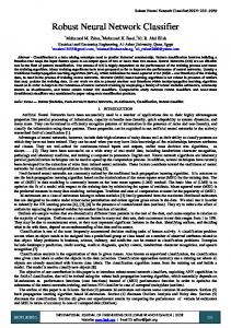
Figure 1: Schematic diagram of automatic encoder model.

Hidden layer (h) Weight (w) Visual layer (v)

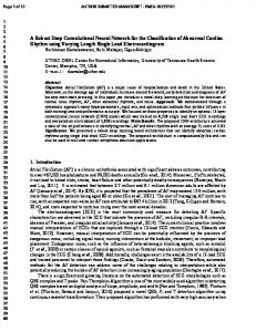
Figure 2: Schematic diagram of restricted Boltzmann machine.

2. Background In this article, we use two kinds of state-of-the-art deep learning models, that is, DAE and RBM [25, 26]. 2.1. Denoising Autoencoder (DAE). Generally, the structure of AE [27] is shown in Figure 1. Here, the whole system consists of two networks, that is, encoder and decoder. Its purpose is to make the reconstruction layer output as similar to the input as possible. The coding network will code and calculate the input x and then reconstruct the result h to r by the decoder. And denoising automatic coding is developed according to the automatic coding, it will learn a more robust representation of the input signal and has stronger generalization ability than ordinary encoders by adding noise to the training data. 2.2. Restricted Boltzmann Machine (RBM). As shown in Figure 2, RBM network has two layers [28, 29]. Here, the first layer is the visual layer (v), also called the input layer, which consists of 𝑚 visible nodes. And the second layer is the hidden layer (h), that is, the feature extraction layer, and it consists of 𝑛 hidden nodes. If V is known, then 𝑃(ℎ/V) = 𝑃(ℎ1 /V) ⋅ ⋅ ⋅ 𝑃(ℎ𝑛 /V) and all hidden nodes are conditional independent. Similarly, all the visible nodes are also conditional independent when the hidden layer h is known, the nodes within the layer are not connected, and the nodes from different layers are fully connected.

3. The Proposed Text Classifier 3.1. Denoising Deep Neural Network (DDNN) 3.1.1. Framework. Here, a DDNN is designed using DAE and RBM, which can effectively reduce the noise while extracting the feature.

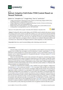
The input of the DDNN model is a vector with fixed dimension. Firstly, we conduct the training by the denoising module composed of two layers, named DAE1 and DAE2, using unsupervised training methods. Here, only one of them is trained each time, and each training can minimize the reconstruction error for the input data, that is, the output of the previous layer. Because we can calculate the encoder or its potential expression based on the previous layer 𝑘, so the (𝑘 + 1)th layer could be processed directly using the output of the 𝑘th layer, until all the denoising layers are trained. The operation of this model is shown in Figure 3. After being processed through the denoising layer, the data enters the portion of RBM, which can further extract the feature that is different from the denoising autocoder layer. The feature extracted after this part will be more representative and essential. Figure 4 is the diagram for the RBM feature extraction. This part is constructed by stacking two layers of RBM. Training can be conducted by training RBM from low to high as follows. (1) The input of bottom RBM is the output of the denoising layer. (2) The feature extracted from the bottom RBM is taken as the input of the top RBM. Because RBM can be trained quickly by contrastive divergence (CD) learning algorithm [30], this training framework avoids the high complexity calculation of directly getting a deep network with one training by dividing it into multiple RBMs training. After this training, the initial parameter values of some pretraining models are obtained. Then, a backpropagation (BP) NN is initialized using these parameters; the network parameters are fine-tuned by the traditional global learning algorithm using the dataset with tags. Thus, the function can converge to the global optimal point. The reason for choosing DAE here is that, in the process of text classification, data will be inevitably mixed into different types and intensity of noise, which tends to affect the training of the model, resulting in deterioration of the final classification performance. DAE is a preliminary extraction of the original features, and its learning criteria is noise reduction. In the pretraining stage, adding a variety of different strength and different types of noise signals to the original input signal can make the encoding process obtain better stability and robustness. It is shown in Figure 5. Moreover, the reason for choosing RBM is that RBM is characterized by the fact that it can simulate the discrete distribution of arbitrary samples and it is very suitable for feature expression when the number of hidden layer units is sufficient. 3.1.2. Implementation. The DDNN model consists of four layers, that is, DAE1, DAE2, RBM1, and RBM2. The layer v is both visual layer and the input layer of the DDNN model. Each document in this article is represented by a fixed dimension vector, where 𝑊1 , 𝑊2 , 𝑊3 , and 𝑊4 represent the connection weight between the layers, respectively. In addition, ℎ1 , ℎ2 , ℎ3 , and ℎ4 represent each hidden layer corresponding to the output layers DAE1, DAE2, RBM1, and

4

Scientific Programming High-level text ℎ4 representation RBM2

··· W4 ···

···

ℎ3

RBM1

ℎ2

DAE2

ℎ1

Noise DAE1 reduction module

W3 ···

···

W2 ···

···

W1 v

···

···

Low-level Text representation

Figure 3: Schematic diagram of denoising deep neural network.

DAE noise reduction

ℎ3

RBM ℎ2

noise signal

reconstructed signal

Figure 5: Noise reduction with DAE.

ℎ1

training the model parameters. Here, RBM energy function is defined as 𝑛 𝑚

𝑚

𝑛

𝑖=1 𝑗=1

𝑗=1

𝑖=1

𝐸 (V, ℎ) = −∑ ∑𝑤𝑖𝑗 ℎ𝑖 V𝑗 − ∑ 𝑏𝑗 V𝑗 − ∑𝑐𝑖 ℎ𝑖 . x

Figure 4: Illustration of feature extraction in RBM.

RBM2, respectively. DAE2 layer is the output layer of the denoising module, and also the input layer of the two-layer RBM module. RBM2 is the output layer of the DDNN model which represents the feature of the document, and it will be compared with the visual layer v. This layer is the highlevel feature representation of the text data. The subsequent text classification task is also addressed on the basis of this vector. For all nodes, there is no connection between the same layer nodes, but the nodes between those two layers are fully connected. Specifically, the introduction of the energy model is to capture the correlation between variables, while optimizing the model parameters. Therefore, it is important to embed the optimal solution problem into the energy function when

(1)

Here, (1) represents the energy function of each visible node and hidden node connection structure. Among them, 𝑛 is the number of hidden nodes, 𝑚 is the number of visible layer nodes, and 𝑏 and 𝑐 are the bias of visual layer and hidden layer, respectively. The objective function of the RBM model is to accumulate the energy of all the visible nodes and the hidden nodes. Therefore, it is necessary for each sample to count the value of all the hidden nodes corresponding to it, so that the total energy can be calculated. The calculation is complex. An effective solution is to convert the problem into probabilistic computing. The joint probability of the visible and the hidden node is 𝑃 (V, ℎ) =

𝑒−𝐸(V,ℎ) . ∑V,ℎ 𝑒−𝐸(V,ℎ)

(2)

By introducing this probability, the energy function can be simplified, and the objective of the solution is to minimize the energy value. There is a theory in statistical learning that the state of low energy has higher probability than high energy, so we maximize this probability and introduce the

Scientific Programming Text preprocessing module

5 Feature learning module

Classification identification module

Figure 6: The architecture of a classifier.

free energy function. The definition of free energy function is as follows: FreeEnergy (V) = − ln ∑𝑒−𝐸(V,ℎ) . ℎ

(3)

Therefore, 𝑃 (V) =

𝑒FreeEnergy(V) , 𝑍 = ∑𝑒−𝐸(V,ℎ) , 𝑍 V,ℎ

(4)

where 𝑍 is the normalization factor. Then, the joint probability 𝑃(V) can be transformed into ln 𝑃 (V) = −FreeEnergy (V) − ln 𝑍.

(5)

The first term on the right side of (5) is the negative value of the sum of the free energy functions of the whole network, and the left is the likelihood function. As we described in the model description, the model parameters can be solved using maximum likelihood function estimation. Here, we first construct a denoising function module for the original features. It is mainly composed of a DAE. The two-layer DAE is placed at the bottom of the model so as to make full use of the character of denoising. The input signal can be denoised by reconstructing the input signal through unsupervised learning, so that the signal entering the network is purer after being processed by the encoder. Then the impact of noise data on the subsequent construction of the classifier will be reduced. The second module is developed using DBN. It is generated through RBM; then the ability of feature extraction in this model will be improved. Furthermore, the model can obtain the complex rules in the data, and the high-level features extracted are more representative. In order to achieve better sorting results, we use the extracted representative feature as an input for the final classifier after further extraction using RBM. Considering the complexity of the training and the efficiency of the model, a two-layer DAE and a two-layer RBM will be used. 3.2. Text Classification Using DDNN. Here, the final DDNNbased text classifier is developed. And there are three key modules in its architecture, as shown in Figure 6. 3.2.1. Text Preprocessing Module. First, the feature words processed here are mapped into the vocabulary form [31–33]. Then, the weights are counted using TF-IDF (term frequency, inverse document frequency) algorithm [34]. In addition, using vector to represent the text is implemented. Meanwhile, it is also normalized.

3.2.2. Feature Learning Module. The DDNN mentioned in Section 3.1 is used to implement feature learning. 3.2.3. Classification Identification Module. In this module, we use Softmax classifier in classification, and its input is the feature which is learned from the feature learning module. In the classifier, the hypothetical text dataset has 𝑛 texts from 𝑘 categories, where the training set is expressed as {(𝑥(1) , 𝑦(1) ), (𝑥(2) , 𝑦(2) ), . . . , (𝑥(𝑛−1) , 𝑦(𝑛−1) ), (𝑥(𝑛) , 𝑦(𝑛) )} and 𝑥(𝑖) represents the 𝑖th training text, and 𝑦 represents different categories (𝑦(𝑖) ∈ {1, 2, . . . , 𝑘 − 1, 𝑘}). The main purpose of the algorithm is to calculate the probability of 𝑥 belonging to the tag category, for the given training set 𝑥. Here, that function is as shown in 𝑃 (𝑦(𝑖) = 1 | 𝑥(𝑖) ; 𝜃) [ ] [𝑃 (𝑦(𝑖) = 2 | 𝑥(𝑖) ; 𝜃)] [ ] ] ℎ𝜃 (𝑥(𝑖) ) = [ [ ] .. [ ] . [ ] (𝑖) (𝑖) [𝑃 (𝑦 = 𝑘 | 𝑥 ; 𝜃)] 𝑇 𝑖

𝑒𝜃1 𝑥

=

1 𝑇 (𝑖) ∑𝑘𝑗=1 𝑒𝜃𝑗 𝑥

(6)

[ 𝑇 (𝑖) ] [ 𝜃2 𝑥 ] [𝑒 ] [ ] [ . ]. [ . ] [ . ] [ ] 𝜃𝑘𝑇 𝑥(𝑖) 𝑒 [ ]

Each subvector of vector ℎ𝜃 (𝑥(𝑖) ) is the probability value that 𝑥 belongs to different tag categories, and the probability value is required to be normalized, so that the sum of probability value of all the subvectors is 1. And 𝜃1 , 𝜃2 , . . . , 𝜃𝑘−1 , 𝜃𝑘 ∈ R𝑛+1 represents the parameter vectors, respectively. After getting 𝜃, we can obtain the previously assumed function ℎ𝜃 (𝑥). It can be used to calculate the probability value that text 𝑥 belongs to each category. The category which has the biggest probability value is the final classified result by the classifier algorithm.

4. Simulation Results and Discussions In this article, simulations are conducted in two steps. First, we analyze the key parameters that affect the performance of the DAE and the RBM models (the basic components of DDNN model) and implement the simulation with appropriate parameters. Second, we compare the DDNN with NB, KNN, SVM, and DBN using the data with noise and the data without noise and verify the effectiveness of the proposed DDNN. 4.1. Evaluation Criterion of Text Classification Results. For the text classification results, we mainly use the accuracy as a classification criterion. This index is widely used to evaluate the performance in the field of information retrieval and statistical classification. If there are two categories of information in the original sample, there are a total of 𝑃 samples which belong to

6

Scientific Programming

category 1, and category 1 is positive. And there are a total of 𝑁 samples which belong to category 0, and category 0 is negative. After the classification, TP samples that belong to category 1 are divided into category 1 correctly, and FN samples are divided into category 0 incorrectly. And TN samples that belong to category 0 are divided into category 0 correctly, FP samples are divided into category 1 incorrectly. Then, the accuracy is defined as Accuracy =

TP . TP + FP

(7)

Here, the accuracy can reflect the performance of the classifier. The recall is defined as Recall =

FN TP =1− . TP + FN 𝑃

(8)

It can reflect the proportion of the positive samples classified correctly. The 𝐹-score is defined as 𝐹-score =

2 × Recall × Accuracy . Recall + Accuracy

(9)

It is a comprehensive reflection of the classification of data. 4.2. Dataset Description. In our simulations, we test the algorithm performance using two news datasets, namely, 20Newsgroups and BBC news datasets. The 20-Newsgroups dataset consists of 20 different news comment groups in which each group represents a news topic. There are three versions in the website (http://qwone .com/∼jason/20Newsgroups/). And we select the second version, that is, a total of 18846 documents, and the dataset has been divided into two parts, where there are 11314 documents for the train set and 7532 documents for the test set. The distribution of the 20 sample details can be found in that website. Note that, in our simulations, the serial number of those 20 labels varies from 0 to 19. The dataset of BBC news consists of several news documents on the BBC website (http://www.bbc.co.uk/news/business/market data/overview/). The dataset includes a total of 2225 documents corresponding to five topics, that is, business, entertainment, politics, sports, and technology. Similarly, we randomly select 1559 documents for train set, and 666 documents for a test set. 4.3. Simulation Results. All the simulations are conducted according to the following. The operating system is Ubuntu 16.04. The hardware environment is NVIDIA Corporation GM204GL [Tesla M60]. The software environment is Cuda V8.0.61 and cuDNN 5.1. Deep learning framework is Keras, while using sklearn and nltk toolkits. 4.3.1. Impact of Parameters. For all deep learning algorithms, the parameter tuning greatly affects the performance of simulation results. For the DDNN, the parameters which we

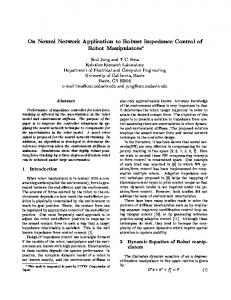
mainly adjust include the plus noise ratio of the data, the number of hidden layer nodes, and the learning rate. In order to test the robustness of the DDNN, we set the plus noise ratio of the training set to 0.01, 0.001, and 0.0001. The result are shown in the Table 1. As shown in Table 1, the stability of the model can be guaranteed within the range of plus noise ratio (0.01, 0.001), but when the plus noise ratio is too high, that is, higher than 0.1, the data will be damaged especially for the sparse data, and it will affect the classification performance. Moreover, the performance of the classifier to robust feature extraction will be weakened if the plus noise ratio is too low. Hence, we set the plus noise ratio finally to 0.001. After we conduct the simulation, we set the noise factor as 0.01, 0.02, 0.03, 0.04, and 0.05 to verify the denoising performance of the proposed model. The number of the input layer nodes is fixed according to the result of the weight using TF-IDF algorithm. Since the main purpose of DAE is to reconstruct original data, we set the numbers of the input layer nodes and output layer nodes to the same value. Because the number of the hidden layer nodes is unknown, we set the numbers of the two hiddenlayer nodes in DAE to 1600 and 1500, 1700 and 1500, and 1800 and 1500, respectively. In addition, the numbers of the two hidden-layer nodes in RBM are set as 600 and 100, 700 and 100, and 800 and 100, respectively. Then, we conduct the simulation. And we set the learning rate to 0.1, 0.01, and 0.001. The results are shown in Table 2. As shown in Table 2, the performance of the DDNN model will be better when the numbers of two hidden-layer nodes are set to 1700 and 1500 for DAE and 700 and 100 for RBM, respectively. And the learning rate should be set to 0.01. 4.3.2. Comparisons and Analysis. In this article, we compare our DDNN model with NB, KNN, SVM, and DBN models. In text preprocessing, we select the frequency of the first 2000 words to simulation and set batch size with 350. Compared with the DDNN model (two-layer DAE and twolayer RBM) proposed in this article, the DBN model is also set to four layers. The number of iterations in the pretraining phase is 100, and the model updating parameter is 0.01. Here, we take the BBC news dataset for an example to show the process of training. From Figures 7 and 8, we can see that, with the increase of epoch, the loss of training is decreasing and the accuracy is increasing towards test datasets, which shows that the effect of training is well. Table 3 compares the results of DDNN with other models using the BBC news dataset and Table 4 compares them using the 20-Newsgroups dataset. Moreover, we compare these models in consideration of different types of data, including the data without noise and the data with a noise factor of 0.01, 0.02, 0.03, 0.04, and 0.05. Here, it is noted that, for each vector of text extracted, the standard normal distribution of noise factor multiplication is added. If a dimension is less than 0, it is directly set to 0. In this article, the accuracy rate (Accuracy), recall rate (Recall), and 𝐹-Score are observed to evaluate the performance of classifier. Take the calculation of Accuracy, for example. Towards each classifier, we firstly calculate the accuracy of each category according to the metric (7) and

Scientific Programming

7 Table 1: Text classification performance of DDNN with different plus noise ratio. Noise factor

Plus noise ratio

0.00 0.7530 0.7536 0.5379

0.001 0.01 0.1

0.01 0.7529 0.7561 0.5310

0.02 0.7479 0.7550 0.5270

0.03 0.7450 0.7542 0.5179

0.04 0.7349 0.7443 0.5027

0.05 0.7287 0.7378 0.4978

Table 2: Text classification performance of DDNN with different parameters. Learning rate

DAE

RBM

1600 1700 1800 1600 1700 1800 1600 1700 1800

0.01

0.02

0.03

1500 1500 1500 1500 1500 1500 1500 1500 1500

600 700 800 600 700 800 600 700 800

100

1.8

90

1.6

Accuracy 0.9640 0.9700 0.9686 0.9655 0.9654 0.9670 0.9625 0.9627 0.9491

100 100 100 100 100 100 100 100 100

1.4

80

1 Loss

Accuracy (%)

1.2 70 60

0.8

50

0.6

40

0.4

30

0.2

20

0 0

20

40

60 Epoch

80

100

120

Figure 7: The test accuracy in the training process for BBC news dataset.

then compute the average of these subaccuracies as the result. The simulation data is the optimal classification result after running many times. After comparing DDNN model with shallow submodel, including KNN and SVM, from those analysis results in Tables 3 and 4, DDNN achieves a better performance. The reason is that when the training set is sufficient, the DDNN can be fully trained, so that the parameters of the network itself can reach the optimal value as much as possible to fit the distribution of training data, and the high-level features extracted from the underlying features are more discriminative for the final classification function. Compared with the DBN model, DDNN first uses the DAE model to train the classification results more accurately in the case that the two layers of the model are the same (they

0

20

40

60

80

100

120

Epoch

Figure 8: The test loss in the training process for BBC news dataset.

are all four layers). This is because the first two layers in the DDNN model are with DAE, which can effectively reduce the impact of noise data, and the DDNN model can be more flexible to adjust the parameters. On the other hand, due to the use of DAE as the initial layer, the dimension of data can also be reduced preliminary. As shown in Tables 3 and 4, the classification performance of NB, KNN, and SVM is obviously decreased when the dataset is adjusted with noise factor, and the DNNN has better antinoise effect for only about 1% decline. Furthermore, Table 5 shows the running time of different models. We can easily find that, for each sample, the NB classifier holds the shortest running time and SVM classifier holds the longest running time. Meanwhile, it can be seen that

8

Scientific Programming Table 3: Text classification performance with different models using BBC news dataset. Classifier

Accuracy

Recall

𝐹-score

NB KNN SVM DBN DDNN NB KNN SVM DBN DDNN NB KNN SVM DBN DDNN

0.00 0.9659 0.9375 0.9715 0.9462 0.9700 0.9655 0.9354 0.9715 0.9459 0.9700 0.9657 0.9364 0.9715 0.9460 0.9700

0.01 0.9560 0.9325 0.9701 0.9434 0.9685 0.9550 0.9324 0.9700 0.9429 0.9685 0.9555 0.9324 0.9700 0.9431 0.9685

Plus ratio noise 0.02 0.03 0.9339 0.8736 0.9284 0.9373 0.9672 0.9583 0.9268 0.9076 0.9582 0.9541 0.9294 0.8453 0.9279 0.9369 0.9670 0.9580 0.9249 0.9039 0.9580 0.9535 0.9316 0.8592 0.9281 0.9371 0.9671 0.9581 0.9258 0.9057 0.9581 0.9538

0.04 0.8186 0.9119 0.9340 0.8789 0.9381 0.7387 0.9114 0.9309 0.8769 0.9399 0.7766 0.9116 0.9324 0.8779 0.9390

0.05 0.7852 0.9260 0.9075 0.8479 0.9286 0.6652 0.9249 0.8964 0.8393 0.9249 0.7202 0.9254 0.9019 0.8436 0.9267

Table 4: Text classification performance with different models using 20-Newsgroup dataset. Classifier

Accuracy

Recall

𝐹-score

NB KNN SVM DBN DDNN NB KNN SVM DBN DDNN NB KNN SVM DBN DDNN

0.00 0.7506 0.6136 0.7598 0.7235 0.7536 0.7483 0.5959 0.7525 0.7149 0.7459 0.7494 0.6046 0.7561 0.7192 0.7497

0.01 0.7274 0.6161 0.7527 0.7207 0.7561 0.6693 0.6000 0.7415 0.7120 0.7500 0.6971 0.6079 0.7471 0.7163 0.7530

Table 5: The running time of different models (ms). Classifier NB KNN SVM DBN DDNN

Dataset BBC news 0.005 0.150 1.660 0.110 0.120

20-Newsgroups 0.006 0.870 12.060 0.180 0.210

the DDNN classifier can keep good classification speed while achieving good classification performance.

Noise factor 0.02 0.03 0.6895 0.6678 0.6213 0.6142 0.7294 0.6968 0.7041 0.6849 0.7550 0.7542 0.5053 0.3526 0.6070 0.6034 0.6966 0.6094 0.6990 0.6826 0.7549 0.7534 0.5832 0.4615 0.6141 0.6088 0.7126 0.6502 0.7015 0.6837 0.7549 0.7538

0.04 0.5887 0.6043 0.6652 0.6562 0.7443 0.2613 0.5939 0.4891 0.6439 0.7439 0.3619 0.5991 0.5637 0.6500 0.7441

0.05 0.4633 0.5978 0.6453 0.6252 0.7378 0.2027 0.5820 0.3833 0.6250 0.7320 0.2820 0.5898 0.4809 0.6251 0.7349

5. Conclusion This article combines the DAE and RBM to design a novel DNN model, named DDNN. The model first denoises the data based on the DAE and then extracts feature of the text effectively based on RBM. Specifically, we conduct the simulations on the 20-Newsgroups and BBC news datasets and compare the proposed model with other traditional classification algorithms, for example, NB, KNN, SVM, and DBN models, considering the impact of noise. It is verified that the DDNN proposed in this article achieves better antinoise performance, which can extract more robust and deeper features while improving the classification performance. Although the proposed model DDNN has achieved satisfactory performance in text classification, the text used in

Scientific Programming the simulations is long-type data. However, considering that there are also some short text data in text classification task, we should address this issue using the model DDNN. Moreover, to further improve the computational performance in the implementation of deep learning methods, in the future we can also design some hybrid learning algorithms by incorporating some advanced optimization techniques, for example, kernel learning and reinforcement learning, into the framework of DDNN, while applying it in some other fields.

Conflicts of Interest The authors declare that there are no conflicts of interest regarding the publication of this paper.

Acknowledgments This research is funded by the Fundamental Research Funds for the China Central Universities of USTB under Grant FRF-BD-16-005A, the National Natural Science Foundation of China under Grant 61174103, the National Key Research and Development Program of China under Grants 2017YFB1002304 and 2017YFB0702300, the Key Laboratory of Geological Information Technology of Ministry of Land and Resources under Grant 2017320, and the University of Science and Technology Beijing-National Taipei University of Technology Joint Research Program under Grant TW201705.

References [1] A. M. Rinaldi, “A content-based approach for document representation and retrieval,” in Proceedings of the 8th ACM Symposium on Document Engineering (DocEng ’08), pp. 106– 109, ACM, S˜ao Paulo, Brazil, September 2008. [2] E. Baykan, M. Henzinger, L. Marian, and I. Weber, “A comprehensive study of features and algorithms for URL-based topic classification,” ACM Transactions on the Web, vol. 5, no. 3, article 15, 2011. [3] P. Langley, W. Iba, and K. Thompson, “An analysis of bayesian classifiers,” in Proceedings of the 10th National Conference on Artificial Intelligence, pp. 223–228, San Jose, Calif, USA, 1992. [4] A. McCallum and K. Nigam, “A comparison of event models for naive bayes text classification,” in Proceedings of the 15th National Conference on Artificial Intelligence—Workshop on Learning for Text Categorization, pp. 41–48, Madison, Wis, USA, 1998. [5] Y. Yang and X. Liu, “A re-examination of text categorization methods,” in Proceedings of the 22nd ACM SIGIR Conference on Research and Development in Information Retrieval (SIGIR ’99), pp. 42–49, Berkeley, Calif, USA, August 1999. [6] S. Godbole, S. Sarawagi, and S. Chakrabarti, “Scaling multi-class support vector machines using inter-class confusion,” in Proceedings of the 8th ACM SIGKDD International Conference on Knowledge Discovery and Data Mining, pp. 513–518, Edmonton, Canada, July 2002. [7] S. L. Y. Lam and D. L. Lee, “Feature reduction for neural network based text categorization,” in Proceedings of the 6th International Conference on Database Systems for Advanced Applications, pp. 195–202, Hsinchu, Taiwan, 1999.

9 [8] M. E. Ruiz and P. Srinivasan, “Hierarchical neural networks for text categorization,” in Proceedings of the 22nd Annual International ACM SIGIR Conference on Research and Development in Information Retrieval, pp. 281-282, Berkeley, Calif, USA, August 1999. [9] L. E. Peterson, “K-nearest neighbor,” Scholarpedia, vol. 4, no. 2, article 1883, 2009. [10] X. Luo, J. Deng, J. Liu, W. Wang, X. Ban, and J. Wang, “A quantized kernel least mean square scheme with entropy-guided learning for intelligent data analysis,” China Communications, vol. 14, no. 7, pp. 127–136, 2017. [11] Y. LeCun, Y. Bengio, and G. Hinton, “Deep learning,” Nature, vol. 521, no. 7553, pp. 436–444, 2015. [12] D. Silver, A. Huang, C. J. Maddison et al., “Mastering the game of Go with deep neural networks and tree search,” Nature, vol. 529, no. 7587, pp. 484–489, 2016. [13] G. E. Hinton, “Deep belief networks,” Scholarpedia, vol. 4, no. 5, article 5947, 2009. [14] P. Smolensky, “Information processing in dynamical systems: foundations of harmony theory,” in Parallel Distributed Processing: Explorations in the Microstructure of Cognition, Volume 1: Foundations, D. E. Rumelhart and J. L. McLelland, Eds., pp. 194– 281, MIT Press, 1986. [15] J. Deng, W. Dong, R. Socher, L. J. Li, K. Li, and F. F. Li, “ImageNet: a large-scale hierarchical image database,” in Proceedings of the IEEE Computer Society Conference on Computer Vision and Pattern Recognition (CVPR ’09), pp. 248–255, Miami, Fla, USA, June 2009. [16] A. Krizhevsky, I. Sutskever, and G. E. Hinton, “ImageNet classification with deep convolutional neural networks,” Communications of the ACM, vol. 60, no. 6, pp. 84–90, 2017. [17] P. Vincent, H. Larochelle, and Y. Bengio, “Extracting and composing robust features with denoising autoencoders,” in Proceedings of the 25th International Conference on Machine Learning, pp. 1096–1103, ACM, Helsinki, Finland, July 2008. [18] P. Vincent, H. Larochelle, and I. Lajoie, “Stacked denoising autoencoders: learning useful representations in a deep network with a local denoising criterion,” Journal of Machine Learning Research, vol. 11, pp. 3371–3408, 2010. [19] G. E. Hinton, “Training products of experts by minimizing contrastive divergence,” Neural Computation, vol. 14, no. 8, pp. 1771–1800, 2002. [20] X. Luo, Y. Xu, W. Wang et al., “Towards enhancing stacked extreme learning machine with sparse autoencoder by correntropy,” Journal of the Franklin Institute, 2017. [21] R. Collobert, J. Weston, and L. Bottou, “Natural language processing (almost) from scratch,” Journal of Machine Learning Research, vol. 12, pp. 2493–2537, 2011. [22] I. Arel, D. C. Rose, and T. P. Karnowski, “Deep machine learning—a new frontier in artificial intelligence research,” IEEE Computational Intelligence Magazine, vol. 5, no. 4, pp. 13–18, 2010. [23] G. E. Hinton, S. Osindero, and Y.-W. Teh, “A fast learning algorithm for deep belief nets,” Neural Computation, vol. 18, no. 7, pp. 1527–1554, 2006. [24] X. Wei and W. B. Croft, “LDA-based document models for adhoc retrieval,” in Proceedings of the 29th Annual International ACM SIGIR Conference on Research and Development in Information Retrieval, pp. 178–185, Seattle, Wash, USA, August 2006. [25] X. Lu, Y. Tsao, S. Matsuda, and C. Hori, “Speech enhancement based on deep denoising autoencoder,” in Proceedings of the 14th

10

[26]

[27] [28]

[29]

[30]

[31]

[32]

[33]

[34]

Scientific Programming Annual Conference of the International Speech Communication Association, pp. 436–440, Lyon, France, August 2013. N. Le Roux and Y. Bengio, “Representational power of restricted Boltzmann machines and deep belief networks,” Neural Computation, vol. 20, no. 6, pp. 1631–1649, 2008. Y. Bengio, “Learning deep architectures for AI,” Foundations and Trends in Machine Learning, vol. 2, no. 1, pp. 1–27, 2009. A. Fischer and C. Igel, “An introduction to restricted Boltzmann machines,” in Proceedings of the 17th Iberoamerican Congress on Progress in Pattern Recognition, Image Analysis, Computer Vision, and Applications, pp. 14–36, Buenos Aires, Argentina, 2012. L. F. Polana and K. E. Barner, “Exploiting restricted Boltzmann machines and deep belief networks in compressed sensing,” IEEE Transactions on Signal Processing, vol. 65, no. 17, pp. 4538– 4550, 2017. R. Karakida, M. Okada, and S.-I. Amari, “Dynamical analysis of contrastive divergence learning: Restricted Boltzmann machines with Gaussian visible units,” Neural Networks, vol. 79, pp. 78–87, 2016. T. Mikolov, I. Sutskever, K. Chen, G. Corrado, and J. Dean, “Distributed representations of words and phrases and their compositionality,” in Proceedings of the International Conference on Neural Information Processing Systems, pp. 3111–3119, Lake Tahoe, Calif, USA, 2013. I. Sutskever, O. Vinyals, and Q. V. Le, “Sequence to sequence learning with neural networks,” in Proceedings of the 28th Annual Conference on Neural Information Processing Systems, pp. 3104–3112, Montreal, Canada, 2014. M. Zhong, H. Liu, and L. Liu, “Method of semantic relevance relation measurement between words,” Journal of Chinese Information Processing, vol. 23, no. 2, pp. 115–122, 2009. L. P. Jing, H. K. Huang, and H. B. Shi, “Improved feature selection approach TFIDF in text mining,” in Proceedings of the International Conference on Machine Learning and Cybernetics, vol. 2, pp. 944–946, Beijing, China, 2002.

Journal of

Advances in

Industrial Engineering

Multimedia

Hindawi Publishing Corporation http://www.hindawi.com

The Scientific World Journal Volume 2014

Hindawi Publishing Corporation http://www.hindawi.com

Volume 2014

Applied Computational Intelligence and Soft Computing

International Journal of

Distributed Sensor Networks Hindawi Publishing Corporation http://www.hindawi.com

Volume 2014

Hindawi Publishing Corporation http://www.hindawi.com

Volume 2014

Hindawi Publishing Corporation http://www.hindawi.com

Volume 201

Advances in

Fuzzy Systems Modelling & Simulation in Engineering Hindawi Publishing Corporation http://www.hindawi.com

Hindawi Publishing Corporation http://www.hindawi.com

Volume 2014

Volume 2014

Submit your manuscripts at https://www.hindawi.com

-RXUQDORI

&RPSXWHU1HWZRUNV DQG&RPPXQLFDWLRQV

 Advances in 

Artificial Intelligence +LQGDZL3XEOLVKLQJ&RUSRUDWLRQ KWWSZZZKLQGDZLFRP

Hindawi Publishing Corporation http://www.hindawi.com

9ROXPH

International Journal of

Biomedical Imaging

Volume 2014

Advances in

$UWLÀFLDO 1HXUDO6\VWHPV

International Journal of

Computer Engineering

Computer Games Technology

Hindawi Publishing Corporation http://www.hindawi.com

Hindawi Publishing Corporation http://www.hindawi.com

Advances in

Volume 2014

Advances in

Software Engineering Volume 2014

Hindawi Publishing Corporation http://www.hindawi.com

Volume 2014

Hindawi Publishing Corporation http://www.hindawi.com

Volume 201

Hindawi Publishing Corporation http://www.hindawi.com

Volume 2014

International Journal of

Reconfigurable Computing

Robotics Hindawi Publishing Corporation http://www.hindawi.com

Computational Intelligence and Neuroscience

Advances in

Human-Computer Interaction

Journal of

Volume 2014

Hindawi Publishing Corporation http://www.hindawi.com

Volume 2014

Hindawi Publishing Corporation http://www.hindawi.com

Journal of

Electrical and Computer Engineering Volume 2014

Hindawi Publishing Corporation http://www.hindawi.com

Volume 2014

Hindawi Publishing Corporation http://www.hindawi.com

Volume 2014