based architecture for Monte Carlo simulations that moni- tors and configures the ... during run-time in order to accommodate the dynamics of the system under ...
A RUN-TIME ADAPTIVE FPGA ARCHITECTURE FOR MONTE CARLO SIMULATIONS Xiang Tian and Christos-Savvas Bouganis Department of Electrical and Electronic Engineering Imperial College London email: {xiang.tian, christos-savvas.bouganis}@imperial.ac.uk ABSTRACT Field Programmable Gate Arrays (FPGAs) are now considered to be one of the preferred computing platforms for high performance computing applications, such as Monte Carlo simulations, due to their large computational power and low power consumption. Unlike other state-of-the-art computing platforms, such as General Purpose Processors (GPPs) and General Purpose Graphics Processing Units (GPGPU), FPGAs can moreover exploit the applications’ requirements with respect to the employed number representation scheme, with the potential to lead to considerable area savings and throughput increases. This work proposes a novel FPGAbased architecture for Monte Carlo simulations that monitors and configures the number representation of the system during run-time in order to accommodate the dynamics of the system under investigation, resulting to a considerable boost on the overall performance of the system compared to a conventional system. In order to evaluate the efficacy of the proposed architecture, the GARCH model from the financial industry is considered as a case study. The results demonstrate that an average of ∼1.35x throughput per resource unit improvement is achieved compared to conventional parallel arithmetic implementation. 1. INTRODUCTION Monte-Carlo simulation of a stochastic process is a procedure that aims to generate random outcomes of that process [1]. In many financial applications the aim is to estimate quantities that are based on some underlying assets, which are modelled as stochastic processes through a system of Stochastic Differential Equations (SDEs). As an analytic solution does not exist in many cases, the Monte-Carlo technique is usually employed to estimate such quantities. Unlike other numerical methods, such as binomial tree, and finite difference methods, Monte-Carlo’s embarrassing parallel nature makes it a good candidate for acceleration by computing platforms that can exploit this characteristic. One of the most important advantages of FPGAs with respect to other existing computational platforms is its capability to operate on a custom number representation scheme.
Significant resource saving and performance boosts have been reported in the literature when an FPGA-based architecture is optimised with respect to its number representation. Both custom floating- and fixed-point arithmetic have been investigated [2][3][4][5] towards these optimisations. However, the investigation of the required number representation for mapping a specific application on an FPGA is performed during the design time. In most of the case, the number representation employed in the final system is selected to accommodate worst-case scenarios, leading to considerable resource overheads compared to the average required number representation scheme.
In this paper, we propose an architecture for Monte-Carlo simulations of SDEs that is able to adapt its number representation during run-time, resulting in considerable throughput increases. The proposed architecture has two key elements; a module that can support run-time reconfiguration of the employed number representation, and a module that can evaluate the quality of the generated results with respect to the chosen number representation. Depending on the result of its evaluation, the system modifies its number representation in order to optimise the objective of the evaluation module. Such a mechanism is acceptable for Monte-Carlo simulations of SDEs when we are interested on the probability density function of the variable under interest rather than its exact final value of each Monte Carlo path.
The rest of the paper focuses on the framework of the proposed system and its analysis. Section 2 introduces the proposed framework that can adaptively change the number representation with respect to the precision requirements of the system under simulation. The proposed quality evaluation metric is given in section 3. Section 4 illustrates the details of several key arithmetic operators employed by the system. Section 5, provides a brief description of the The GARCH model, which is chosen as a case study. Section 6 provides a discussion and analysis on the obtained results.
Control module Real-time Adaptive Monte Carlo simulation engine Evaluation module
Fig. 1. Framework of the Proposed Monte Carlo Simulation Engine
2. PROPOSED MONTE CARLO SIMULATION FRAMEWORK In a Monte Carlo simulation of a stochastic process, a large number of possible outcomes of the variables of interest are generated, through the simulation of many Monte Carlo paths. These paths are dictated by the SDEs that describe the dynamics of the system. In most of the cases, of interest is the probability distribution of the outcome rather the actual final value of each path. Please note that further optimisations can be performed with respect to the employed number representation scheme when information regarding the actual usage of the generated samples is available. This is considered to be out of the scope of this work, as it is of interest to design a general Monte Carlo engine that can drive any function of interest. In this work, a novel Monte Carlo simulation architecture is proposed that consists of a run-time adaptive Monte Carlo simulation engine, which can be reconfigured during run-time in order to perform arithmetic operations with various word-lengths, an evaluation module, which is responsible to measure the quality of the generated results during run-time, and a control module that takes as input the quality of the generated results and decides the appropriate system’s word-length. The proposed architecture is depicted in Fig.1.
3. EVALUATION MODULE As the main task of the Monte Carlo simulation is to capture the probability distribution of a variable of interest, the objective of the evaluation module is to assess whether the estimated probability distribution using a certain number representation scheme converges to the distribution that would be generated when the engine was configured to the full supported precision (i.e. maximum word-length). Thus, a metric is needed to evaluate the quality of the results with respect to the number representation. Possible methods can be based on the statistics of the variables of interest like the first (expectation) and second central moments (variance), or even higher order moments. Moreover, a comparison based on the Probability Density Function (PDF) or Cumulative Distribution Function (CDF) can also be considered as a method of evaluating the quality of the outcome of the system. In this work, the Kolmogorov-Smirnov test (KS test) is adopted, as it provides a measure of the distance of two cumulative distribution functions and can be efficiently mapped onto an FPGA using only a modest amount of resources. Two types of KS test exist; one-sample KS test and twosample KS test. The first one is used to compare a set of samples with a reference probability distribution, and the latter is for the comparison of two sets of samples. As the probability distribution of the variable is unknown, the onesample test cannot be applied. The two-sample KS test is employed in this work, as the comparison between the distribution of the samples from high precision module and low precision module needs to be performed. The KS statistic measures the maximum distance between the empirical distribution functions (EDF) of two sets of samples. For example, denoting by EDF F1 ,n (x ) for n independent and identically distributed (iid) random samples, and EDF F1 ,m (x ) for the other sample set, the KS statistic is given by: Dm,n = sup |F1,m (x) − F2,n (x)|
The Monte Carlo simulation engine consists of many identical modules (sub-engines) that perform a subset of the Monte-Carlo simulation paths. The novel feature of the proposed framework is the ability of the Monte Carlo simulation engine to alter its system number representation during run-time, depending on the impact of the word-length to the quality of the generated results, tuning its characteristics to the actual requirements of the given SDEs that need to be simulated. In this work, the serial arithmetic is investigated as a potential solution for the dynamically reconfigurable computation engine. In order to provide a reference quality measure, the runtime adaptive Monte Carlo engine configures two out of its many modules to the full supported word-length (high precision modules). As such, the system is aware of its performance under full word-length.
(1)
x
where sup is the supremum of the set of distances. Fig. 2 illustrates the KS statistic when samples from a Monte Carlo simulation engine are generated using various word lengths. In this example, a million samples are generated using 16 bits, 24 bits, and 32 bits. The EDF for each case is plotted in the figure. As it is expected, the 32 bits implementation gives the smoothest EDF, and the 16 bits implementation has the largest distance to the EDF of 32 bits implementation. 4. ARITHMETIC OPERATORS This section focuses on the run-time reconfiguration of the Monte Carlo engine with respect to the employed number
tation. For example, a 32 bits addition can be performed on a one bit full adder using 32 clock cycles. Hence, optimal design of the basic arithmetic operators and exploration of the trade-off between the resource consumption and the throughput is essential for the efficacy of the system. 1 16 bits 32 bits 20 bits
0.9
C umulative probability
0.8 0.7 0.6 0.5 0.4 0.3 0.2 0.1 0
0.5
1
1.5
2
Data 0.83
C umulative probability
16 bits 32 bits 20 bits
0.825
0.82
0.815 1.119
1.12
1.121
1.122
1.123
1.124
1.125
1.126
1.127
1.128
Data
Fig. 2. EDF of Samples Generated from modules with different word-lengths.
representation. In this work, the fixed-point number representation is exploited. In order to achieve run-time dynamic reconfiguration with respect to the number representation having minimum overhead, the arithmetic hardware modules are based on serial arithmetic. As the numerical values are represented by digit vectors, it is possible to apply the inputs and deliver the outputs in a one digit at a time fashion, so that all digits of the same numerical operands/results share the same digit lines. Using this method, the wordlength of the system can be changed by having an impact on the number of clock cycles needed by the arithmetic operator to produce a result. Although the throughput of the arithmetic operators is reduced, the resource consumption of the basic operators is largely reduced as the arithmetic operation reuses the hardware resources for each digit in the represen-
Firstly, several issues need to be addressed when employing serial arithmetic. When the product or the sum of two numbers is calculated, the process starts from the least significant bit, as the carry bit needs to be generated and propagated to the next level. However, a square root or division starts by the most significant bit. Therefore, when the calculation of an arithmetic expression under serial arithmetic is required that involves various arithmetic operations, shift registers are necessary in order to change the bit order of the inputs to the components. An alternative method to the above, is to employ online arithmetic [6]. In this case, the bits can be processed starting from the most-significant bit. However, an initial investigation showed that this algorithm exhibits significant control logic overheads in the case of online arithmetic. Thus, in this work, the combination of LSB and MSB arithmetic is adopted. Another issue is the digit size of the basic operators. For instance, to do a 32 bits addition, 1 bit, 4 bits, 8 bits, or 16 bits per clock cycle can be processed typically. Let’s take the 1-bit mode as an example. When calculating a 32 bits addition, 32 clock cycles are needed to get the result. A 32 bits parallel adder can produce one result per clock cycle. However, the resource consumption of a 1-bit adder is approximately 1/32 of a 32 bits parallel adder. Hence, if thirtytwo 1-bit adders are employed, the normalised throughput (bit per silicon area unit) of the serial adder and the parallel adder should be the same, without considering the clock frequency. As the system needs to adapt its wordlength, extra logic is needed. Initial experiments showed that the overhead of the control logic of having a one bit-level configurations is considerable large relative to the resources allocated for the actual operation. Hence, the selected modes of operation for the arithmetic components are 8 or 16 bits, with maximum wordlength of 32 bits. Note that in the following of this paper, these three modes will be named as radix-256 and radix-65536. The following sections provide a detailed description of the three basic arithmetic elements; an adder, a multiplier, and a square root hardware modules.
4.1. Serial Adder A radix-2n serial adder is formed by n 1-bit full adder as shown in Fig.3.(a). Due to space limitations, a radix-16 adder is depicted in Fig.3.(b).
D31-0
x0 y0
c s0
XOR
SUB 15
x1
y
1-bit Full Adder
XOR
x2
s c
y2
Q15
s1
XOR
4-bit Full Adder
s2
XOR
SUB
y3, y2, y1, y0
y1 x
X
R31-30
D29-0
SUB 16
NxM Mul
Q15-14
R30-28
D29-0 D27-0
x3 y3
s3
XOR
(N+M) bits Full Adder s c
SUB 17 z3, z2, z1, z0
SUB
(a)
Q15-13
(b)
Fig. 3. (a) 1-bit serial adder/subtractor. (b) Radix-16 digitserial adder/subtractor.
R29-26
D29-0
SUB 18
Q15-12
(a)
R28-24
D29-0
(b)
Fig. 4. (a) Serial multiplier (b) Square root operator 4.2. Serial Multiplier 5. CASE STUDY Two possible architectures can be considered for a serial multiplier (both using LSB first algorithm); a serial-serial multiplier and serial-parallel multiplier. For the serial-serial multiplier, both operands are used in serial mode. For the serial-parallel multiplier, one of the operands is used in serial mode, and the other one is in the parallel form. It has been showed that the first mode requires more hardware resources and longer delay [6]. Therefore, the serial-parallel multiplier architecture is adopted in this work. Fig.4.(a) shows the architecture of the adopted serial multiplier. In the figure, M is the maximum word length of the operands (both operands have the same word length), and N is the digit size. As shown in Fig.4.(a), X is loaded into the multiplier in the parallel form, and N bits of Y are loaded one per clock cycle. Hence, a N × M multiplier and a N + M full adder are required.
4.3. Square Root For the current case study application, a square root module is required. The result of this operation is then fed to as adder. As it has been mentioned before, when an addition is followed by a square root operation, the bit order need to be changed from LSB first to MSB first. Hence, the operand can be loaded into the operator in parallel form. The adopted square root algorithm is based on the work from [7]. However, instead of shifting one bit per clock cycle as in [7], the shift can be performed by either 8 bits or 16 bits per clock cycle. Hence, for example, the basic element of a radix-16 square root module is shown in Fig.4.(b) (The maximal operation word length is 32 bits in this figure).
The GARCH model [8] is chosen as a case study in order to assess the performance of the proposed architecture. It is one of the most widely used financial models, and as it requires a large amount of computations, its acceleration using specialised hardware is of great interest. 5.1. GARCH Model The GARCH model in financial applications is based on the dynamics of the underlying asset that follows the Brownian motion, which is described as: σ2 )dt + σdz) (2) 2 S is the asset price at time t, S 0 is the asset price at time t + dt, the expected drift rate in S is assumed to be µS for a constant parameter µ. This means that in a short interval of time, given as δt, the expected increase in S is µSδt. The parameter µ is the expected rate of return on the stock, expressed in decimal form. The volatility of the stock price is σ. Moreover, dz is a Wiener process, which is related to dt by the following equation: √ dz = ε dt S 0 = S(1 + (µ −
ε is a random variable with a normal distribution with a mean of zero and a standard deviation of 1.0. In many cases, the volatility of the stock is not constant, as it is assumed by the above model. Actually, in many cases, the stock price and volatility are depended, resulting to the above system to not have a close form solution leading to numerical methods and particularly to Monte Carlo based simulations as the only means to provide a solution for the above problem.
One technique for modelling volatility that has become popular is the GARCH model. The most commonly used one is GARCH (1, 1) where the volatility is given by the following equation: 2 2 σi2 = σ0 + ασi−1 + βσi−1 λ2
(3)
Here α, and β are constants that can be estimated from historical data using maximum likelihood methods. σ0 is the volatility of the stock price at time 0, σi and σi−1 are the volatilities at time i∆t and (i − 1)∆t. λ is a random variable with a normal (Gaussian) distribution with a mean of zero and a standard deviation of 1.0. Note that the random variable in the GARCH model is different from the one used in the describing the evolution of stock prices. The two random variables represent two independent stochastic processes. 6. IMPLEMENTATION AND PERFORMANCE EVALUATION
Cash flow generator
GARCH module Monte Carlo simulation engine (High precision) Random number generator
Monte Carlo simulation engine (Low precision) Random number generator
CDF CDF generation generation
Cash flow generator
GARCH module
KS statistics
KS statistics
CDF generation
Decision module
Monte Carlo simulation engine (Low precision) Random number generator
Cash flow generator
Cash flow generator
GARCH module
GARCH module
Fig. 5. Detailed framework of Monte Carlo simulation based GARCH model. Table 1. Resources Consumption and Frequency
Given the stochastic differential equations (SDEs) that describe the dynamics of the system, multiple Monte-Carlo simulation sub-engines are instantiated based on the serial arithmetic operators that have been mentioned in section 4. The evaluation module’s objective is to compute the histogram of the generated samples from the Monte Carlo simulation kernel. This is performed using a counting bins approach after each sample is produced. This step is straight forward as a fixed-point arithmetic is employed. The required resources consist of an accumulator, which is responsible to generate the histogram and an embedded RAM to store the generated histogram. The depth of the embedded RAM is equal to the number of bins, and the number of bins depends on the maximum word length of the system. Next, a set of time points for performing the monitoring and assessment of the quality of the results is required. At each time point, the histograms of the high precision and low precision modules are fetched from the embedded RAMs and the empirical cumulative distribution functions (EDFs) are calculated, followed by the calculation of the maximum distance between the two EDFs (KS statistic). Note that there is no need to normalise the cumulative sum. Given the KS statistic between the high and low precision modules, named R, a threshold value is needed to be set in order to assess whether the current word-length generates samples that follow a probability density function close to the one that is generated by the high precision module. This is performed by using another high precision module, and calculating the KS statistic between two high precision modules, named P . The objective function used by the control module shown below, where the threshold determines the normalised distance. (R − P )/P
Monte Carlo simulation engine (High precision) Random number generator
(4)
Serial 8
Serial16
Parallel32
Registers
6459
6599
3424
LUTs
15521
22341
10316
LUT-FF pairs
5090
4882
5474
BRAMs
8
8
5
Frequency (MHz)
272
222
211
Please note that the generation of the EDFs does not require stalling the Monte Carlo simulation engine as modern FPGA devices support dual-ported memories. The detailed framework is shown in Fig.5. In this figure, two high precision modules are used to calculate P . Moreover, there are several low precision modules. The results from the low precision modules are used for comparison against the results from one of the high precision module to estimate the value R. The framework of the run-time Monte Carlo simulation engine is implemented using a Virtex6-LX550 chip. The synthesis is done using Xilinx ISE 12.2. Two digit sizes are implemented: 8 bits and 16 bits. Also a reference design based on a 32 bit fixed point arithmetic has been implemented. Please note that the serial versions consist of three reconfigurable modules, where two of them have been configured as high precision modules and one as a low precision module. In order to calculate the normalised throughput, only reconfigurable logic and BlockRAMs are used during the synthesis stage. The resource consumption and the achieved frequency are shown in Table 1. The employed random number generators are from the work in [9]. It is a Mersenne-Twister uniform random number generator followed by an Inverse Cumulative Distribution Function (ICDF) module to produce Gaussian random
1.4
2.4
S16.16 S16.32 S8.8 S8.16 S8.24 S8.32 P32
2
Normalized throughput
Normalized throughput compared to P32
2.2
1.8
1.6
1.4
1.2
1
0.8
1.3 1.25 1.2 1.15 1.1 1.05 Digit size = 8 bits Digit size = 16 bits Maximal throughput of digit size 8 bits Maximal throughput of digit size 8 bits
1 0.95
0.6
0.4 0
1.35
2
4
6
8
10
12
14
16
18
20
Number of low precision MC engines
Fig. 6. Throughput of the Monte Carlo Simulation Engine
samples. Moreover, the random number generator uses parallel arithmetic. Therefore, for instance, one 32 bit random number generator can supply two digit size 16 bits Monte Carlo simulation sub-engines. Given the reported resource consumption and timing report by the synthesis tool, the normalised throughput (results/second/LUT) is estimated. The results are plotted in Fig.6. The number of the Monte Carlo simulation engines is varied in order to show the trend of the achieved normalised throughput. Note that the similar clock frequency of the serial and parallel implementations, removes the impact of clock frequency on the overall throughput. The “S16.32” legend denotes a configuration with digit size 16 bits, and operating at 32 bits. “P32” denotes a parallel arithmetic of 32 bits. The throughput (results/second/LUT) is normalised to the results of P32 case. Hence, the P32 is indicated by a horizontal line with a normalised frequency of 1. For the case of 16 bits digit size, S16.16 is the maximum throughput that can be achieved where S16.32 is the minimum throughput. As the graph shows, the S16.16 line converges to a value around 1.4. This is because the resource consumption of the S16 implementation is roughly half of the P32 one (considering the control logic for the serial arithmetic, it is a bit more than half), and the frequency of the S16 is slighter higher than P32. Also, the S16.32 line converges to 1.0. However, the S8.24 and S8.32 lines follow a downward trend as the number of sub-engines increases. This is because the overhead of the control logic overtakes any increase in the achieved throughput. In summary, the proposed engines can achieve a range of throughputs depending on their configuration, with some cases producing much
0.9 0.1
0.2
0.3
0.4
0.5
0.6
0.7
0.8
0.9
1
Threshold value
Fig. 7. Actual achieved normalized throughput
higher throughput than the conventional architecture, where in other cases, they achieve a reduced throughput. The actual operation of the system depends on the dynamics of the simulation. As Fig.6. presents only the upper and lower bounds of the throughput, more experiments were constructed to investigate the achieved normalised throughput during an actual simulation, using both digit 8 bits and 16 bits architectures. The only parameter in the proposed framework is the threshold value that controls the switch in the mode of operation of the Monte Carlo engines. It is expected that the normalised throughput will increase along with the increase of the threshold value, as more deviation from the high precision EDF is allowed. The digit size 16 bits architecture can be adaptively configured at 16 and 32 bits. When the value calculated from equation (4) is above the threshold value, the Monte Carlo simulation sub-engines are configured to 32 bits, otherwise they operate at 16 bits. The digit size 8 bits can be configured at 16, 24, 32 bits. Hence there are two stages of decision. When the value calculated from equation (4) is larger than the threshold value, the computing kernel will be configured at 32 bits, if it is between the threshold value and half of the threshold value, the kernel will be configured at 24 bits, otherwise to 16 bits. Fig 7. depicts the obtained results over 10 runs with different parameters of the GARCH model. The x-axis is the threshold value as is defined in equation (4). The obtained results demonstrate that the proposed framework always produces better results than the reference design achieving a boost in the normalised throughput between 10% and 35%.
7. CONCLUSION In this work, a novel run-time reconfigurable Monte Carlo simulation engine has been presented. The proposed framework takes advantage of the flexibility allowed during the estimation of the probability density functions in Monte Carlo based simulations to explore the resource-performance design space. In this work, the run-time reconfiguration is achieved though serial arithmetic and several serial operators have been developed. Moreover, the KS metric is proposed to assess the quality of the generated results. The efficacy of the proposed framework is demonstrated through an example from the financial sector, the GARCH model. The obtained results show that the proposed framework can achieve a boost in the normalised performance between 10% and 35% when operators with the digit size 8 bits and 16 bits are employed compared to a 32 bits parallel arithmetic architecture. Future work will address the further optimisation of the proposed framework when information about the use of the generated results is available. 8. REFERENCES [1] P. Glasserman, Monte Carlo Methods in Financial Engineering (Stochastic Modelling and Applied Probability). Springer, Aug. 2003. [Online]. Available: http://www.amazon.com/exec/obidos/redirect?tag=citeulike0720&path=ASIN/0387004513 [2] A. Kaganov, P. Chow, and A. Lakhany, “Fpga acceleration of monte-carlo based credit derivative pricing,” in Field Programmable Logic and Applications, 2008. FPL 2008. International Conference on, 2008, pp. 329 –334. [3] N. Singla, M. Hall, B. Shands, and R. Chamberlain, “Financial monte carlo simulation on architecturally diverse systems,” in High Performance Computational Finance, 2008. WHPCF 2008. Workshop on, 2008, pp. 1 –7. [4] X. Tian and K. Benkrid, “Design and implementation of a high performance financial monte-carlo simulation engine on an fpga supercomputer,” in ICECE Technology, 2008. FPT 2008. International Conference on, 2008, pp. 81 –88. [5] ——, “Fixed-point arithmetic error estimation in monte-carlo simulations,” Reconfigurable Computing and FPGAs, International Conference on, vol. 0, pp. 202–207, 2010. [6] M. D. Ercegovac and T. Lang, Digital Arithmetic, 1st ed., ser. The Morgan Kaufmann Series in Computer Architecture and Design. Morgan Kaufmann, June 2003. [Online]. Available: http://www.worldcat.org/isbn/1558607986 [7] Y. Li and W. Chu, “A new non-restoring square root algorithm and its vlsi implementations,” in Computer Design: VLSI in Computers and Processors, 1996. ICCD ’96. Proceedings., 1996 IEEE International Conference on, Oct. 1996, pp. 538 –544. [8] J.-C. Duan, “The garch option pricing model,” Mathematical Finance, vol. 5, no. 1, pp. 13–32, 1995. [Online]. Available: http://ideas.repec.org/a/bla/mathfi/v5y1995i1p13-32.html
[9] X. Tian and K. Benkrid, “Implementation of the longstaff and schwartz american option pricing model on fpga,” Journal of Signal Processing Systems, pp. 1–13, 2010, 10.1007/s11265010-0550-1.