A SARS Multiband Spectrum Sensing Method in ... - IEEE Xplore

19th European Signal Processing Conference (EUSIPCO 2011)

Barcelona, Spain, August 29 - September 2, 2011

A SARS MULTIBAND SPECTRUM SENSING METHOD IN WIDEBAND COMMUNICATION SYSTEMS USING RSG Bashar I. Ahmad, Andrzej Tarczynski and Mustafa Al-Ani School of Electronics and Software Engineering, University of Westminster 115 New Cavendish Street, London W1W 6UW {email: [email protected]; [email protected]} ABSTRACT This paper introduces a multiband spectrum sensing method that can accomplish the sensing task using sampling rates considerably lower than the ones demanded by the uniformsampling-based techniques. It utilises nonuniform sampling in conjunction with an appropriate spectral analysis tool. The approach is referred to as Spectral Analysis of Randomized Sampling (SARS), namely for the Random Sampling on Grid (RSG) scheme. The statistical characteristics of the adopted periodogram-type estimator are presented and the effects of the cyclostationary nature of the processed communication signals on SARS are addressed. Reliability guidelines that ensure the credibility of the sensing procedure amid a sought system performance are derived. Unlike a number of previously reported nonuniform sampling schemes e.g. Total Random Sampling (TRS), the RSG provides safeguards making it more suitable for implementation in hardware. Numerical examples testify the presented analytical results. 1.

INTRODUCTION

Spectrum sensing involves scanning part(s) of the radio spectrum in search for a meaningful activity e.g. a transmission. The envisioned Cognitive Radio (CR) technology has initiated intensive research into effective spectrum sensing techniques [1, 2]. To perform the sensing task using uniformsampling-based DSP without prior knowledge of the incoming signal’s frequency support, the sampling rates should be at least twice the total monitored frequency range(s) regardless of the spectral activity within [3]. Otherwise aliasing would introduce irresolvable detection problems. In the event of examining wide bandwidths, such a constraint can pose a challenge to the system designer where high sampling rates and treating large quantities of data are required [1, 2, 4, 5]. Such stringent demands can be beyond the capability of the commercially available data acquisition devices i.e. Analogue to Digital Converters (ADCs). In this paper, we proposed a method that can reliably sense the spectrum using an arbitrary low-rate nonuniform sampling and appropriate processing of the signal-a methodology known by Digital Alias-free Signal Processing (DASP) [6]. Operating at low sampling rates, can exploit the sensing device resources e.g. power more efficiently and/or evade the possible need for a specialized hardware. Here, the scenario where the overseen wide bandwidth consists of a number of disjoint spectral subbands is considered i.e. Multiband Spectrum Sensing (MSS). In such scenarios, MSS approaches that are based on nonparametric spectral analysis are viewed as adequate low-complexity options [1, 2]. A periodogram-type

© EURASIP, 2011 - ISSN 2076-1465

estimator, a tool that retained its popularity [1, 2], is deployed in this study for the SARS purpose. Low rate tactful sampling and processing aimed at mitigating the aliasing/bandwidth limitation of uniform sampling has triggered an immense interest in the emerging Compressive Sensing (CS) trend e.g. [4, 5]. Reconstructing the sampled signal is inherently an integrated part of CS that imposes sampling frequencies above the Landua rate i.e. twice the effective bandwidth of the present signal not the monitored bandwidth. The difference between the latter two can be significant with low spectrum occupancy e.g. some CR systems. However, reconstruction might not be needed in certain tasks e.g. MSS. CS capability and performance comes at a considerable computational cost accompanying the optimisations it entails. Whilst the simplicity, low computational load and not having a lower limit on the utilised sampling rate are the main advantages of the proposed SARS method over CS or other approaches e.g. spectrum-blind sampling [7]. A SARS technique that relies on the TRS scheme was studied in [8]. Related work in the literature on MSS with SARS can be found therein. It was shown that MSS can be carried out with arbitrary low sampling rates. However, any two or more points of a TRS sequence can be arbitrarily close i.e. TRS requires infinitely fast ADC(s). Other randomised sampling schemes for DASP e.g. Poisson sampling suffer from a similar defect [6]. In this paper, an alternative sampling scheme, i.e. RSG, is adopted. It guarantees a minimum distance between any two sample points, requests lower sampling rates than TRS and is better suited for the use of FFTlike algorithms [9]. It is more practical and efficient. The statistical characteristics of SARS with RSG are presented here and the impact of the cyclostationary nature of communication signals is scrutinised. Unlike [8, 9], the nonstationarity of the processed signal is not circumvented – a widely adopted practice in the literature [1, 2]. It is shown to have repercussions especially on the SARS accuracy i.e. abrupt deterioration at certain frequency points. We provide guidelines to ensure that the MSS procedure meets the sought detection probabilities. The system subbands can have different power levels e.g. due to the propagation channel effect(s). This is distinct from [8, 9] where the surveyed subbands are assumed to be of equal power levels and a generic Chebychev’s inequality parameter depicts the MSS performance. 2. MULTIBAND SPECTRUM SENISNG 2.1 System Model and Problem Formulation The frequency range of interest encompasses L disjunct contiguous subbands each of width BC i.e. the monitored

1219

bandwidth B = [ fin , fin + B] of a predefined fin has a width B = LBC . The incoming multiband signal at the sensing device is: x(t ) = ∑ m =1 xm (t ) where M is the unknown number M

of the concurrently active subbands and xm (t ) is the transmission corresponding to the m-th active subband. The samples of the zero mean wide sense cyclostationary signal x(t ) are contaminated with additive white Gaussian noise with variance PN i.e. y (tn ) = x(tn ) + n(tn ) . Due to adverse system conditions e.g. propagation-channel effects, the individual transmissions xm (t ) ’s can be of various power levels. Our objective in this study is to devise an algorithm that is capable of scanning the overseen bandwidth B and unveiling the active subbands. It should operate at rates significantly lower than the theoretical minimum permissible uniform sampling one 2B (not always achievable) [3]. Let xk (t ) be the incoming linearly modulated continuoustime signal corresponding to one of the system subbands: xk (t ) = ∑ n =−∞ an , k si , k (t , n) + ∑ n =−∞ bn , k sq , k (t , n) . +∞

+∞

The coefficients {an, k }n∈

and {bn, k }n∈ are the transmitted

H1, k :

Xˆ e ( f k ) ≥ γ k

and

σ b2, k

respectively.

sq , k (t , n) = [ pq , k (t + nTS , k )cos(2π fC , k t + 0.5π )] ⊗ hk (t ) , ⊗ de-

notes the convolution operation and hk (t ) is the propagation channel impulse response over the k -th subband with a central frequency fC , k and symbol rate f S , k = 1/ TS , k . Each of pi , k (t ) and pq , k (t ) are the baseband shaping filter(s) in the

inphase and quadrature branches respectively. 2.2 Random Sampling on Grid RSG scheme selects randomly N sampling instants inside an analysis time window T r = [ tr , tr + T0 ] . Let α = N / T0 denote the average sampling rate. The RSG samples are restricted to a specific finite set of time-instants that are equally spaced and placed within T r . They form an underlying uniform sampling grid whose sampling rate and total number of samples are given by f g = 1/ Tg and N g respectively. Any of the grid points can be selected only once, i.e. without reN placement, with equal probability where CN possible sampling sequences of length N exist. g

2.3 Adopted Sensing Technique The approach adopted here deploys a periodogram-type tool: N n =1

nal windows of length T0 are considered in this paper. The sensing technique adopted here comprises two steps: 1) estimating the magnitude spectrum at selected frequency point(s) and 2) comparing the magnitude(s) to pre-set threshold(s). We recall that the signal’s exact PSD is not the target. We seek inspecting one frequency point per subband (positioned at its centre) to establish its status i.e. L spectral points are calculated. This can be achieved by performing spectral analysis within a suitably short time windows i.e. low resolution spectrograph. As shown in [8], T0 ≥ 1/ BC offers a practical guideline for choosing the analysis window. The sensing problem can be formulated as: Xˆ e ( f k ) < γ k

σ a2, k

y (tn ) w(tn )e − j 2π ftn

2

N ( N − 1) μ (2)

to estimate a detectable frequency representation of x(t )

(3)

to enhance the estimation accuracy. This evokes shifting T r and the aligning of w(t ) . Non-overlapping uncorrelated sig-

H 0, k :

Whilst si , k (t , n) = [ pi , k (t + nTS , k )cos(2π fC , k t )] ⊗ hk (t ) ,

∑

K Xˆ e ( f ) = ∑ r =1 X e ( tr , f ) / K

(1)

symbols with variances

X e ( tr , f ) = ( N g − 1)T0

of a periodogram-type estimator is known to be of the same order as its expected value [10]. To reduce this uncertainly, we average a K number of X e ( tr , f ) estimates where:

(4)

k = 1,2,… L

where γ k is the threshold, H 0,k hypothesis signifies the absence of an activity in subband k and H1,k exhibits the presence of an activity. Below we show that (3) can deliver reliable spectrum sensing routine provided the adequate selection of the grid density, average sampling rate α and K . 3.

STATISTICAL CHARACTERTISCS OF SARS

We present the mean and variance of (3) to assess its adequacy for the MSS pursuit and its accuracy. 3.1 Targeted Frequency Representation By introducing a random variable cn which takes a value of “1” if the n-th grid point is considered and “0” otherwise where Pr {cn = 1} = N / N g and Pr {cn = 0} = ( N g − N ) / N g , it can be shown that C ( tr , f ) = E [ X e ( tr , f )] is: C ( tr , f ) =

( N g − N ) PS ( tr ) + ( N g − 1) PN ( N − 1) N g f g

+

E ⎡⎣P d ( tr , f ) ⎤⎦ fg μ

(5)

, PS ( tr ) = ∑ n =1 E[ x 2 (nTg )]w2 (nTg ) / μ is the windowed signal Ng

power and P d ( tr , f ) =

∑

Ng n =1

x(nTg ) w(nTg )e

− j 2π fnTg

2

. It can

be noticed from (5) that C ( tr , f ) comprises a constant frequency-independent component and the expected value of a discrete-time periodogram [10]. The former would not overshadow any distinctive feature(s) of E[P d ( tr , f )] related to active transmission(s). Below, we show that E[P d ( tr , f )] serves as a detectable spectral component and is independent of tr at selected frequency points i.e. f k ’s in (4).

from N RSG noisy samples y (tn ) ’s captured within T r . It is noted that estimating the signal’s exact PSD is not the objective and a frequency representation that enables sensing is sufficient. Tapering function w(t ) is used to suppress spec-

Provided that f g is chosen such that X W ( f ) X W ( f − nf g ) = 0

tral-leakage where μ = ∑ n =1 w2 (nTg ) . The standard deviation

for n ≠ 0 , n ∈ , where X W ( tr , f ) = ∫t∈T x(t ) w(t )e − j 2π ft dt then:

Ng

1220

r

E[P d ( tr , f )] = f g2 ∑ n∈ E[P ( tr , f − nf g )] i.e. avoid aliasing

I RG ( tr , f ) = ∑ n =1 y (tn ) w(tn )sin(2π ftn − θ ( tr , f )) are uncorre-

within B whilst P ( tr , f ) =| X W ( tr , f ) |2 . Bandpass sampling strategy [3] can be utilised to select f g . Thus, the adequacy

lated for every f . Similar to [9], X e ( tr , f ) have a chisquare distribution with two degrees of freedom according to Central Limit Theorem (CLT) and σˆ e2 ( f ) = var{ X e ( tr , f )}/ K can be shown to be closely approximated at f k ’s in (4) by:

of (2) for the MSS purpose is mandated by E[P ( tr , f )] . First, +∞

w(t )e − j 2π ft dt , H m ( f ) = ∫ hm (t )e− j 2π ft dt ,

let W ( f ) = ∫

t∈T r

Pi , m ( f ) = ∫

+∞

−∞

σˆ e2 ( f k ) = 2ηˆk Dk2 / K + 2( N g − N ) [ PSA + ν PN ] Dk [( N − 1) f g K ]

−∞

Pq , m ( f ) = ∫

pi , m (t )e− j 2π ft dt ,

+∞

−∞

N

+ ( N g − N ) 2 ⎡⎣ PSA′ + 2ν PSA PN + ν 2 PN2 ⎤⎦ [( N − 1) 2 f g2 K ]

pq , m (t )e − j 2π ft dt ,

(12)

Pi , m ( f ) = H m ( f + fC , m ) Pi , m ( f ) , Pi , m ( f ) = H m ( f − f C , m ) Pi , m ( f ) ,

where ν = ( N g − 1) /( N g − N ) , PSA′ = ∑ r =1 PSA2 ( tr ) / K , 0.5 ≤ ηˆ ≤ 1

Pq , m ( f ) = H m ( f + f C , m ) Pq , m ( f ) , Pq , m ( f ) = H m ( f − f C , m ) Pq , m ( f ) .

and Dk = E[P d ( tr , f k )]/ f g μ ( E[P d ( tr , f )] is time-invariant

Noting the bandpass nature of H m ( f ) over the m-th subband and assuming fC , m >> BC , using (1) we obtain: E[P ( tr , f )] = 0.25∑ m=1σ a2,m f S ,m Fi ,m ( tr , f ) + σ b2,m f S ,m Fq ,m ( tr , f ) (6)

at the assessed frequency points). The first component in (12) forms a substantial part of the estimator’s variance. Here we show that ηˆk can acquire its highest possible value ηˆk = 1 notably degrading the estimation accuracy for certain signals.

Fi , m ( tr , f ) = ∑ n =−∞ ⎡⎣ Pi , m ( f − f C , m ) Pi*, m ( f − f C , m + nf S , m )

Note that λC ( tr , f ) = E[ R 2 ( tr , f )] and λS ( tr , f ) = E[ I 2 ( tr , f )]

M

+∞

+ Pi , m ( f + f C , m ) Pi*, m ( f + f C , m + nf S , m ) ⎤⎦ ⊗ ⎡⎣W ( f )W * ( f − nf S , m ) ⎤⎦ Fq , m ( tr , f ) = ∑ n =−∞ ⎡⎣ Pq , m ( f − f C , m ) Pq*, m ( f − f C , m + nf S , m )

(7)

N

(8)

. The baud rate is related to the bandwidth BW , m of the baseband

shaping

BW , m ≤ BC .

filter(s)

It

by:

implies:

0.5BW , m < f S , m ≤ BW , m where

Pi , m ( f ) Pi , m ( f + nf S , m ) = 0

and

Pq , m ( f ) Pq , m ( f + nf S , m ) = 0 if n ∉ {−1,0,1} . Hence, the compo-

nents of the summation in (7) and (8) are zero when n = ±1 as the assessed frequency points f k ’s in (4) are placed at/near the middle of the subbands i.e. at those frequencies: E[P ( tr , f )] = f S ,m 4

M

∑σ m=1

+σ b ,m

2 a ,m

2

{

{⎡⎢⎣ P ( f − f i ,m

C ,m

2 2 2 ) + Pi ,m ( f + fC ,m ) ⎤ ⊗ W ( f ) ⎥⎦

⎡ P ( f − f ) 2 + P ( f + f ) 2⎤ ⊗ W( f ) 2 C ,m q ,m C ,m ⎢⎣ q ,m ⎥⎦

}

}

(9)

. Therefore, P ( tr , f k ) and subsequently P ( tr , f k ) embodies a distinctive distinguishable feature depicted by the Fourier transform of the transmission filter(s) shaped by the propagation channel and is time-invariant at/near the centre of the subbands. This results in the expected value of (3): ( N − N ) PSA + ( N g − 1) PN E[P d ( tr , f k )] Cˆ ( f k ) = g + (10) d

( N − 1) f g

fg μ

where PSA = ∑ r =1 PS ( tr ) / K . Thus, Xˆ e ( f k ) in (3) is an admisK

sible tool to unveil the presence of an active transmission regardless of the used sampling rate α (a suitable underlying grid density is presumed as described above). 3.2 Estimator’s Accuracy The accuracy of estimation of Cˆ ( f ) via (3) can be related to the variance via Chebychev’s inequality [8, 9]. We can write: 2 2 X e ( tr , f ) = ( N g − 1)T0 ⎡⎣ RRG ( tr , f ) + I RG ( tr , f ) ⎤⎦ N ( N − 1) μ (11) where the phase shift θ ( tr , f ) is selected such that each of RRG ( tr , f ) = ∑ n =1 y (tn ) w(tn ) cos(2π ftn − θ ( tr , f )) and N

which results in: λC ( tr , f ) + λS ( tr , f ) = E[P d ( tr , f )] where R ( tr , f ) = ∑ n =g1 x ( nTg ) w( nTg )cos(2π fnTg − θ ( tr , f )) and

+∞

+ Pq , m ( f + f C , m ) Pq*, m ( f + f C , m + nf S , m ) ⎤⎦ ⊗ ⎡⎣W ( f )W * ( f − nf S , m ) ⎤⎦

K

I ( tr , f ) = ∑ n =g1 x ( nTg ) w( nTg )sin(2π fnTg − θ ( tr , f )) . Thus, N

λC2 ( tr , f ) + λS2 ( tr , f ) = η ( tr , f ){E[P d ( tr , f )]}2

(13)

where 0.5 ≤ η ( tr , f ) ≤ 1 whilst ηˆk is the average η ( tr , f k ) along the K signal windows at the f k frequency point. From (13), it can be seen that Γ( tr , f ) = λC ( tr , f ) − λS ( tr , f ) dictates the η ( tr , f ) value i.e. if λC ( tr , f k ) ≈ λS ( tr , f k ) we get Γ( tr , f k ) ≈ 0 , η ( tr , f k ) ≈ 0.5 and ηˆk ≈ 0.5 which is the case for wide sense stationary signals as in [9]. It can be easily noticed that Γ( tr , f ) = 2ψ ( tr , f ) . For the legitimate f g value (see Section 3.1): Pi , m ( f ) Pi , m ( f − nf g ) = 0 for n ≠ 0 ( n is an integer) and similarly for the quadrate filter(s). Assuming that the analysis window tends to infinity to illustrate the impact of the cyclostationarity on (12) i.e. W ( f ) tends to a Dirac delta δ ( f ) , ψ ( tr , f ) is defined by: ψ ( tr , f ) = 0.5cos(2θ ( tr , f )) f g2 ∑ n∈

∑

M m =1

Gm ( tr , f − nf g ) (14)

for the M concurrently active subbands where Gm ( tr , f ) = 0.125 f S , m ⎡ξ1 ( f )∑ l =−∞ δ ( f − f C , m − 0.5lf S , m ) ⎣ +∞ + ξ 2 ( f )∑ l =−∞ δ ( f + fC , m − 0.5lf S , m ) ⎤ ⎦ ξ1 ( f ) = H m2 ( f ) ⎡⎣σ a2, m Pi ,2m ( f − fC , m ) − σ b2, m Pq2, m ( f − fC , m ) ⎤⎦ +∞

(15) (16)

ξ 2 ( f ) = H m2 ( f ) ⎡⎣σ a2, m Pi ,2m ( f + fC , m ) − σ b2, m Pq2, m ( f + fC , m ) ⎤⎦ . (17)

Formulas (14)-(17) show that ψ ( tr , f ) can have nonzero values concentrated at frequencies equal to multiples of half of the symbol rate f S , m and belong to the m-th active subband. Such peaks are experienced when any mismatch between σ a2, m Pi , m ( f ) and σ b2, m Pq , m ( f ) takes place generating discrepancies between λR ( tr , f ) and λI ( tr , f ) . This yields abrupt surges in the estimation variance at the corresponding frequencies according to (12) and (13). This phenomenon is

1221

clearly observed with BPSK signals where only an inphase branch is present. Thus η ( tr , f k ) and subsequently ηˆk can tend to their maximum values causing noticeable deterioration in the estimator’s accuracy in case f k falls at/near the f n = 0.5nf S , m frequency(ies) that belong(s) to the m-th active transmission band. Whilst for QAM and QPSK, typically σ a2, m Pi , m ( f ) = σ b2, m Pq , m ( f ) i.e. ψ ( tr , f ) ≈ 0 and ηˆk = 0.5 is commensurate. If no beforehand knowledge is available on the modulation scheme characteristics, ηˆk = 1 should be selected to avoid any unforeseen anomalies in the estimator’s performance. Therefore, the accuracy of (3) can be affected by the signal’s cyclostationarity and any processing task that relies on the spectral analysis, e.g. MSS, should consider such aspect. The accuracy of the above analysis was verified through numerical examples (not shown here). 4. RELIABLE SPECTRUM SENSING The reliability of a sensing technique is reflected by its ability to meet a sought system behaviour that is commonly expressed by the Receiver’s Operating Characteristic(ROC) [1]. Here, we procure the reliability recommendations to ensure that the proposed method satisfies the sought ROC probabilities of a targeted subband indexed by k in the sequel. 4.1 Reliability Recommendations According to CLT, Xˆ e ( f ) can be approximated by a normal distribution at every f for large K (in practice K ≥ 20 suffices[1]). This is validated below by simulations even for K < 20 . Thus, (3) can be compactly written as: Xˆ e ( f k ) ∼ N (m0, k ,σ 0,2 k ) , m0, k = C ( f k ) and σ 0, k = σˆ e ( f k ) for H 0, k and similarly Xˆ e ( f k ) ∼ N (m1, k ,σ 1,2 k ) for H1, k . From (4),

the probability of a false alarm in the k -th subband is: Pf , k (γ k ) = Pr{H1, k H 0, k } = Q[(γ k − m0, k ) / σ 0, k ]

(18)

and that of correct detection is: Pd , k (γ k ) = Pr{H1, k H1, k } = Q[(γ k − m1, K ) / σ 1, k ]

Formula (22) is a conservative lower bound on the number of needed window averages to fulfil the pursed detection probabilities. It is a function of the average sampling rate, signal to noise ratio, the active subbands power ratios and the uniform grid density. The recommendation demonstrates the trade-offs between the number of estimate averages and the deployed sampling rate in a particular scenario. It can be used to decide on the average sampling rate for a number of estimate averages possibly demanded by practical constraints such as latency in a continuous processing environment. The impact of the nonstationary nature of the processed signals is manifest by ηˆk (see Section 3). Formula (22) affirms that the sensing task can be accomplished with arbitrarily low sampling rates at the expense of longer signal observation windows. A numerical example is presented below to verify its accuracy. If more than one subband is targeted, the user should survey their individual α / K requirements via (22). Aiming to detect a weak or high performance subband(s) would request more K and/or higher α compared to a stronger or lower performance ones. The thresholds needed in (4) for each subband is set by (20). The spectral peaks Dn ’s for n = 1, 2,… L can be learnt a priori when the transmissions are known to be present as in [1, 2]. Such knowledge can be exploited to determine φk and the parameters needed for calculating the thresholds in (20) e.g. for the severe cases when the maximum expected subbands activity is incurred. Correlated and/or overlapping signal windows can be easily incorporated into the analysis above by using existing results in the literature on variance reductions e.g. Welch periodograms [10]. Cooperation among a number of possible sensing devices can be implemented at a network level higher than the studied physical level. 4.2 RSG versus TRS and Uniform Sampling RSG becomes identical to TRS as the underlying grid rate tends to infinity, and (22) emerges as:

{

2 KTRS ≥ Q −1 ( Δ) KTRS −Q −1 ( ) KTRS + 2 KTRS + 2ηˆk

(19)

for a preselected threshold value γ k where Q( z ) is the tail probability of normal distribution. In practice, the user typically specifies: Pf , k ≤ Δ and Pd , k ≥ . From (18) and (19): γ min, k ≤ γ k ≤ γ max, k m1, k − m0, k ≥ Q −1 ( Δ )σ 0, k − Q −1 ( )σ 1, k

(21)

which defines the reliability condition of the MSS. The mean and standard deviation values in (18) and (21) can be directly obtained from (10) and (12) respectively. Adopting a conservative approach, it can be shown that (21) produces:

2

(23)

where KTRS = 2 BCφk N [1 + SNR ]/( N − 1)α . Whilst, the scheme becomes uniform sampling when all the grid points are considered and the recommendation reduces to: −1

{

2 KUS ≥ Q −1 (Δ) KUS −Q −1 ( ) KUS + 2 KUS + 2ηˆk

(20)

γ min, k = m0, k + Q −1 ( Δ)σ 0, k , γ max, k = m1, k + Q −1 ( )σ 1, k ( f k ) and

}

}

2

(24)

where KUS = 2 BCφk SNR −1 / fUS and fUS is the uniform sampling rate that is appropriately set to avoid aliasing within B . Comparing RSG and TRS, it can be shown that K < KTRS for a reasonable f g . Formulas (22)-(24) offer a means to evalu-

and SNR = PSA / PN . Whilst, φk = PSA / PSA, k is the ratio of the

ate the requirements of each of their corresponding sampling scheme and assess the benefits/complexity of SARS with RSG. They can be used to examine the number of needed signal samples of each of the schemes. This can be a crucial factor as the adopted MSS involves discrete-time Fourier transform or an optimized version. Unlike TRS and Poisson sampling, RSG maintains a minimum distance between the collected samples i.e. Tg and is better suited for FFT-like

total signal power to that occupying the targeted subband.

algorithms e.g. zero filling of unused grid points [6].

{

K ≥ Q −1 (Δ) K −Q −1 ( ) K 2 + 2 K + 2ηˆk

}, 2

(22)

K = 2 BCφk N ( N g − N ) ⎡⎣1 + ( N g − 1) SNR −1 ( N g − N ) ⎤⎦ N gα ( N − 1)

1222

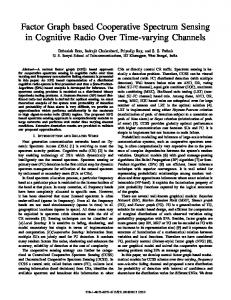
5. SIMULATIONS Consider a multiband system comprising L = 40 contiguous subbands where BC = 2.5 MHz and they are located in B = [1.65,1.75] GHz. QAM signals are transmitted over the

active subbands ( i.e. ηˆk = 0.5 ) noting that the SNR is 1.6 dB. The grid rate f g = 220 MHz which satisfies X W ( f ) X W ( f − nf g ) = 0 if n ≠ 0 ( n is an integer) is used

along with a Blackman window of length T0 = 1 us. A sampling rate α = 68 MHz is decided, it is significantly lower than the minimum valid uniform sampling rate i.e. 220 MHz. The aim is to fulfil the detection requirements of the targeted subband centred at f31 . The user specified: Pf ,31 (γ 31 ) ≤ 0.05 and Pd ,31 (γ 31 ) ≥ 0.96 . For φ31 = 2.12 (four simultaneously active subbands), K ≥ 11 estimates need to be averaged in (3) to meet the sought system performance according to (22) . In Fig. 1a, we show the ROC of SARS with RSG method for a threshold sweep and in Fig. 1b the probabilities are displayed for the threshold values in (20). The results were obtained from 10000 independent simulations. Fig. 1 confirms the moderately conservative nature of the given reliability recommendations where the desired performance is achieved for K ≥ 11 upon satisfying the inequality in (21). This also affirms that the assumptions undertaken did not have noticeable effect on the accuracy of results including the normality one. Thus, the proposed technique here provides nearly 67% saving on the sampling rate and 20% reduction on the number of processed samples in comparison to uniform sampling. It also gives nearly 20% saving on the latter compared to TRS. It is clear that SARS with RSG delivers notable savings in terms of the complexity of the sensing procedure, especially in low spectrum occupancy environment e.g. CR in certain frequency ranges. Formulas (22)-(24) allow the user to examine the possible benefits of utilizing SARS in a given scenario. For illustration purposes, Fig. 2 depicts the targeted subband’s ROC if the present transmissions were of a BPSK type and ηˆ31 = 0.5 i.e. the cyclostationarity effect(s) on the estimation accuracy is ignored. It is clear from the figure that the detection method has failed to deliver the requested probabilities for K = 11 . This demonstrates the impact of the nonstationarity of communication signals on SARS and that precautions should be taken. If we chose ηˆk = 1 in (22), we would attain K ≥ 15 which mends the MSS response (see Fig. 2). 6. CONCLUSIONS The proposed SARS with RSG is a reliable spectrum sensing technique that offers substantial savings on the sampling rate compared to the uniform-sampling-based ones. It can use considerably low sampling rates i.e. ease the stringent sampling requirements of the wideband MSS procedure. The cyclostationary nature of communication signals is shown to cause degradation in the SARS quality and should be countered. The provided reliability guidelines, which ensure fulfilling the detection probabilities, illustrate the trade-offs between the sampling rate and the length of the

observation window. This paper serves as an impetus and prompts further research into DASP-based MSS methods. REFERENCES [1] Z. Quan, S. Cui, H. V. Poor, and A. H. Sayed, "Collaborative Wideband Sensing for Cognitive Radios," IEEE Signal Processing Magazine, vol.25, pp.60-73, 2008. [2] J. Ma, G. Y. Li, and B. H. Juang, "Signal processing in cognitive radio," Proceedings of the IEEE, vol.97, pp.805-823, 2009. [3] R. Vaughan, N. Scott, and D. White, "The Theory of Bandpass Sampling," IEEE Trans. on Sig. Proces, pp.1973-1984, 1991. [4] Y. Polo, Y. Wang, Pandharipande, and G. Leus, "Compressive Wide-band Spectrum Sensing," in proc.IEEE Int. Conf. on Acous., Speech and Sig. Proces., 2009, TX, pp.2337-2340. [5] M. Mishali and Y. C. Eldar, "Blind Multiband Signal Reconstruction: Compressed Sensing For Analog Signals," IEEE Trans. on Signal Process., vol.57, pp.993-1009, 2009. [6] I. Bilinskis, Digital Alias-free Signal Processing, New York, John Wiley and Sons, 2007. [7] R. Venkataramani and Y. Bresler, "Perfect Reconstruction Formulas and Bounds on Aliasing Error in Sub-Nyquist Nonuniform sampling of Multiband Signals," IEEE Trans. On Info. Theory, vol.46, pp.2173-2183, 2000. [8] B. I. Ahmad and A. Tarczynski, "Reliable Wideband Multichannel Spectrum Sensing Using Randomized Sampling Schemes," Signal Processing, vol.90, pp.2232-2242, 2010. [9] B. I. Ahmad and A. Tarczynski, "Wideband Spectrum Sensing Technique Based on Random Sampling on Grid: Achieving Lower Sampling Rates," Digital Signal Processing, 2011. [10]M. H. Hayes, Statistical Digital Signal Processing and Model ing, John Wiley & Sons, 1996.

Fig. 1, Detection probabilities of the targeted subband. (a) ROC for

a threshold sweep; asterisk is (0.05,0.96) , (b) γ min,31 ≤ γ 31 ≤ γ max,31 .

1223

Fig. 2, ROC for the BPSK case; asterisk (0.05,0.96) .