SUs using dedicated wireless spectrum sensor networks (WSSNs). In this paper we focus on the sensing channel assignment problem in WSSNs and formulate ...
2010 16th International Conference on Parallel and Distributed Systems
SCAS: Sensing Channel ASsignment for Spectrum Sensing Using Dedicated Wireless Sensor Networks Min Gao∗ , Lan Cheng† , Yunhuai Liu† and Lionel Ni∗† ∗ Hong Kong University of Science and Technology † Shenzhen Institutes of Advanced Technology, Chinese Academy of Science őŖ
Abstract—Spectrum sensing is essential for the success of the cognitive radio networks. In traditional spectrum sensing schemes, Secondary Users (SUs) are responsible for the spectrum sensing which could be very time and resource consuming. It leads to a great deal of inefficiency in spectrum usage and introduces many practical challenges. To tackle these challenges and leverage the spectrum opportunity more efficiently, we propose a new system that provides a spectrum sensing service for SUs using dedicated wireless spectrum sensor networks (WSSNs). In this paper we focus on the sensing channel assignment problem in WSSNs and formulate the problem as a Sensing Effectiveness Maximization Problem (SEMP). We prove that SEMP is NP-complete under the ideal case, and show that the more challenges arises in real environments. To address the issues, we systematically study the design tradeoff and critical factors when maximizing the sensing effectiveness. Based on these study results we propose a Sensing Channel ASsignment algorithm (SCAS). We conduct test-bed empirical investigations as well as comprehensive simulations. Performance evaluation results show that for both the scenarios of given deployments and manual deployments, SCAS is able to sense more channels to improve the sensing effectiveness. The improvement is up to 300% and the average improvement is 150% compared with other simple alternatives.
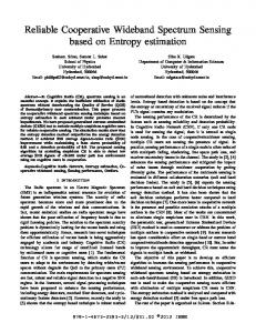
ŅŦŵŦŤŵŦťġţŰŶůťŢųź
ńũŢůůŦŭġIJ őŖ
œŦŢŭġţŰŶůťŢųź
őŖ
ńũŢůůŦŭġIJ
œŦŢŭġţŰŶůťŢųź ŅŦŵŦŤŵŦťġţŰŶůťŢųź
ĩŢĪįġłŭŭġŴŦůŴŰųŴġŢųŦġŢŴŴŪŨůŦťġŵŰġŴŦůŴŦġŰůŦġ ŤũŢůůŦŭġŸŪŵũġŵũŦġţŦŴŵġŴŦůŴŪůŨġŢŤŤŶųŢŤź
Fig. 1.
ńũŢůůŦŭġij
ĩţĪį ŔŦůŴŰųŴġŢųŦġŢŴŴŪŨůŦťġŵŰġŵŸŰġŤũŢůůŦŭŴġ ŸŪŵũġŢġţŦŵŵŦųġŴűŦŤŵųŶŮġŶŵŪŭŪŻŢŵŪŰů
Motivation example for multiple PU spectrum sensing scheduling
Many research works have been done for spectrum sensing. In most of the existing works, the spectrum sensing is conducted by SUs, presenting many many limitations and practical constraints in real environments. First, the typical SU devices do not support simultaneous spectrum sensing and accessing. As the spectrum sensing brings no benefits for the spectrum usage, extra hardware is needed if SUs want to fully exploits spectrum opportunity. Efficient scheduling of the spectrum sensing and accessing is also a challenging issue [4]. Second, because of the hardware limitations, the individual sensing results may contain notable errors. To meet the mandatory requirements on sensing accuracy, different SUs should work cooperatively [5]. As different SUs often work for different organizations, additional management costs and communication overhead among SUs are inevitable. Information sharing and privacy protection are also challenges. To tackle these issues, a more promising approach is to provide a spectrum sensing service using wireless sensor networks [6] [7]. A large number of low-cost, well-designed and carefully controlled sensors are deployed to the field, forming a network and dedicatedly providing the spectrum information for users. SUs subscribe the service, leveraging sensors to acquire the sensing information. They do not need to conduct the spectrum sensing, which could be very time and resource consuming, and can focus on the spectrum accessing only. In this way, a much higher spectrum usage is expected. In addition, many practical challenges in spectrum sensing such as the security, privacy and information sharing become minor. We refer such a system to as Wireless Spectrum Sensor Networks (WSSNs) and an illustration of the system architecture is given in Fig. 1. The success of the WSSNs highly depends on the spec-
I. I NTRODUCTION As the scarce spectrum resources are allocating out, the cognitive radio networks (CRNs) [1] have received increasing research attentions for the target of more efficient usage of the wireless spectrum. Different from the traditional wireless networks in which the spectrum are allocated and used in an exclusive manner, in CRNs, the valuable spectrum resources are used in a shared manner. In CRNs, a primary user (PU), the license holder of a spectrum, can always use the spectrum when needed. the secondary users (SUs) have no license but can opportunistically use the licensed spectrum if they cause no harmful interference to the PU. To guarantee the accessing priority of the PUs, the draft of IEEE 802.22 standard [2] is established to regulate the behaviors of SUs. It is required that SUs must evacuate the primary spectrum immediately when the licensed PUs return. Thus, whenever the SUs are trying to utilize the primary channel for communications1 , they must acquire enough information of the real-time spectrum usage. IEEE 802.22 requires that PUs must be detected within 2 seconds, and specifies that both the misdetection probability PM D and the false alarm rate PF A should be no more than 0.1 [3]. 1 In this paper we will use the spectrum and channel interchangeable if no otherwise specified
1521-9097/10 $26.00 © 2010 IEEE DOI 10.1109/ICPADS.2010.118
łųŦŢŴġŤŢůġţŦġ ŶŴŦťġţźġŔŖŴ
492
trum availability information that provided. To quantify the usefulness of the spectrum information and meter the attractiveness of a sensing service, in this paper we define a metric accumulated sensing effectiveness. It measures the areas and channels that can be used by SUs for a given sensing result (formal definitions will be in later Sec. IV). The accumulated sensing effectiveness is inherently different the sensing effectiveness of individual channels. As exampled in Fig. 1, one approach for the assignment is to assign all sensor in a single channel (Fig.1(a)). This approach is accurate that yields the best sensing effectiveness for this channel. An alternative approach is to assign the sensors to different channels, say two in Fig. 1(b). In the second approach, sensing effectiveness of either channel may be less than that of the first one due to more sensing errors. However, a better accumulated sensing effectiveness is expected because two channels are sensed simultaneously. Sensing more channels may get no further benefits as the effectiveness is degraded too much that compromises the gains from sensing more channels. To provide such a service, typically we only have a limited number of sensors because of the budget control. The system design goal is therefore to maximize the accumulated sensing effectiveness using this limited number of sensors. Towards this goal there are several key issues that need to be addressed: (1) the set of simultaneously sensed channels; 2) the assignment of the sensors to each channel, and; 3) the sensing algorithm for each channel. In a previous work [8], we comprehensively studied the last issue and proposed a voronoibased declaration calibration algorithm together with a SVMbased boundary detection algorithm. In this paper, we will focus on the other two questions and investigate the sensing channel assignment for sensors. The channel assignment has several key challenges to be addressed. The first challenge is that individual sensing results may contain notable errors. The relation between the number of sensors and the sensing effectiveness is not clear yet. The second challenge is that there is a nature tradeoff between the sensing effectiveness of individual channels and the number of sensed channels. We prove that even under the ideal case, the problem is NP-complete. The third challenge is that the sensing effectiveness is closely related to the deployment of the sensors. Yet we have little knowledge about which deployment will yield the best results. To tackle these challenges, we first study the key factors that have the critical impact on the sensing effectiveness of individual channels. With such understanding, we propose a sensing channel assignment algorithm SCAS, seeking the maximization of the accumulated sensing effectiveness with a limited number of sensors. To the best of our knowledge, this is the first work in literature that dedicatedly focuses on the channel assignment for spectrum sensing using WSSNs. Our contributions are highlighted as following. • We identify the unique features and challenges of spectrum sensing using WSSNs. We formulate the problem as the Sensing Effectiveness Maximization Problem (SEMP) and prove that SEMP is NP-complete in ideal cases.
To study SEMP in practice, we conduct extensive empirical studies to verify a spectrum sensing model based on a test-bed of 10 Telosb nodes [9]. Experimental results show that the theoretical Raylei model can appropriately describe the sensing behaviors of individual nodes. The gap between the model and the practice is no more than 10% on average. • We systematically study the key factors of the sensing for individual channels in practice. The sensor deployments with high sensing effectiveness are well featured and analyzed. • Based on the results, we propose a Sensing Channel ASsignment algorithm (SCAS). We conduct comprehensive simulation experiments to evaluate the performance of SCAS. Experimental results show that SCAS can improve the accumulated sensing effectiveness by up to 300% compared with a naive randomized assignment. The rest of the paper is organized as follows. In Sec. II we give a review of the related work. In Sec. III we give some preliminary information for the spectrum sensing. The formal definition of the problem will be presented in Sec. IV as well as some analytic results. In Sec. V, we present the proposed SCAS in details and evaluate its performance in Sec. VI. In the last section we conclude this work and point out some possible future work directions. •
II. R ELATED W ORK Spectrum sensing plays an important role in CRNs. The current research works for spectrum sensing can be categorized into to two main classes. One is SU-based sensing schemes, and the other class is based on sensor network to provide the spectrum sensing services. For the first class of SU-based spectrum sensing, it can be further categorized into three groups. The first group of works focus on studying possible spectrum detection methods. Cabric et. al. [10] presents an experimental study of energy detection method for spectrum sensing. Energy detection utilizes the Received Signal Strength (RSS) to judge the appearance of the PUs. According to the results, energy detection is faster but the sensing accuracy is relatively lower. In the work [11], Cordeiro et. al studies the feature detection method which analyzes the received signals to distinguish the PUs from other SUs. The sensing accuracy of feature detection is much higher than that of energy detection, while experiences more sensing time. Noticing the truth that a SU cannot support simultaneous spectrum sensing and accessing, Kim et. al [4] proposes inband spectrum sensing algorithm which forms an optimal group of SUs and scheduling different detection methods among them so as to achieve the best performance. All these works focus on the sensing accuracy of individual nodes, and the third majority group of works attempt to improve the sensing accuracy by fusion the sensing results of a number of sensors. Noticing the benefits of dedicated spectrum sensing services, WSSNs was proposed. Projects Sendora [6] and CROPS [12] suggest a possible infrastructure. In our previous work [8],
493
Error of boundary detection ε
Primary Network
Central Station of Wireless Spectrum Sensor Network
in S f o pe r m ct ati rum on qu sp er ec Pr o y tr u v m ide i n th fo e rm at io n
Cognitive Radio Network
1.0 0.8 0.6 10dB, Real 10dB, Rayleigh 15dB, Rayleight 15dB, Real 20dB, Rayleigh 20dB, Real
0.4 0.2
0
10
20
30
40
50
Normalized Received Signal Strength
Fig. 3. The CDF of individual detected energy comparing to Rayleigh fading model; the x-axis is the random variable to denote the detected energy level, and different curves represents those of different P (d)
Fig. 2. System architecture of spectrum sensing using dedicated wireless sensor networks
while such reliable communications are left for the designers of the sensors. The station makes calculations based on the collected reports and provides the information to SUs that subscribe the services. In the next, we describe the sensing model that features the sensing behavior of individual nodes.
we formalize the problems as a boundary detection problem with erroneous inputs. Though there have been extensive studies on the boundary detection in wireless sensor networks, the majority of the existing works assumed the corrected inputs (e.g., [13] [14] [15]). In particular, Krishnamachari et. al. [14] studied the boundary detection with certain erroneous inputs. They however assumed that the erroneous sensors are surrounded by corrected ones and did not consider the erroneous sensors near the boundary.
B. Empirical studies of Rayleigh model We conduct comprehensive field studies to evaluate the effectiveness of Rayleigh model in real environments. Since currently there are no off-the-shelf spectrum sensors available, we use the 2.4G ISM band to emulate the licensed band. We build a test-bed with one 802.11g wireless router emulating the behavior of the PU channel and 10 TelosB sensor nodes [9] [17] to sense PU spectrum. We inject backlog traffics for the router so that the spectrum is very likely to be fully utilized. The 10 Berkeley TelosB sensor nodes are configured in the same spectrum as the router. Each sensor measures 1000 samples of the spectrum and report the sensed RSS to a laptop. Fig. 3 depicts the CDF of RSS at three locations. Though there is a gap between the field measurement and the ideal RSS level calculated by Rayleigh model, the trends of the two are consistent and the gap is acceptable. The errors are no more than 10%.
III. P RELIMINARY In this section, we give a formal formulation of the problem we want to tackle in this paper. Firstly, we describe the system architecture of the WSSNs. Secondly, we empirically verify the rayleigh signal model that we are using for individual sensing results. Finally, basing on these models, we formally formulate the problem, state the key challenges and give some analysis results. A. System architecture In WSSNs, a number of static spectrum sensors are deployed to an application field for spectrum sensing purposes. Each sensor node can sense only one spectrum channel at a time. Sensors will based on their sensing declare whether the PU of the sensed spectrum is present at the location or not. In this paper we use energy detection sensing method [10], while the proposed algorithms can be applied for other detection methods (e.g., feature detection [11]) with minor extensions. PU channels are modeled as an ”on/off” resource. For one location and one channel, if it is covered by a PU, we say that there is an ”on” status at this location for the channel. Otherwise, it is an ”off” status. We allow the co-existence of multiple PUs at the same time in the field, while different PUs must be distributed to different channels. We have this restriction because PUs have the exclusive priority to use their licensed spectrums. For a given primary channel, even if it is allocated to multiple PUs, the PUs must be far away enough so as to avoid harmful interference in between. Sensors sense the assigned channel, and reports the sensing results to a central station through a specific control channel (e.g., using a 2.4G ISM band [16]). We assume the transmissions between the sensors and the central station is reliable,
IV. P ROBLEM S TATEMENT AND A NALYSIS In this section, we give the formal statement of the problem and present analysis results for the problem. A. Concepts and Notations Without loss of the generality, we assume the application field A is a rectangle. The left-down corner of A is set as the coordinate origin. The multiple PUs are working on exclusive channels, each of which covers a certain area of A. When sensors, denoted as V = {v0 , v1 , ..., vn }, have been deployed to the field, we assume sensors are able to gather their precise locations by GPS devices or other localization algorithms (e.g., [18]). As different sensors are assigned to different channels to sense, we use nk to denote the number of sensors assigned in the k-th channel. Suppose totally there are T channels for sensing, called candidate sensing channels. Clearly we have n=
t ∑ k=1
494
nk , t < T
(1)
Misdetection area LMD Real boundary
Sensing utility per channel
Sensed covered area L R
1
Sensed whitespace area LS
PU
0.9
0.8
0.7
0.6 Triangular Hexagon Uniform Random
0.5
25
100
225
400
625
900
Number of sensors False-alarm area LFA
Sensed boundary
Fig. 5. Sensing effectiveness for single channels under different deployments 0.3
Sensing utility per channel
Fig. 4. An example of the sensing results; the sensed and real boundaries as well as the four sub-areas are illustrated
where t is the total number of simultaneously sensed channels. When the sensors assigned to each channel have been determined, the issue then becomes how to reduce the sensing error of each sensed channel. This problem has been extensively studied by our previous work [8] and in this paper we will use the results directly.
P(MD), Triangular P(MD), Hexagon P(MD), Uniform P(MD), Random P(FA), Triangular P(FA), Hexagon P(FA), Uniform P(FA), Random
0.25
0.2
0.15
0.1
0.05
25
100
225
400
625
900
Number of sensors
Fig. 6. Misdetection and false alarm percentage under different deployments
Definition Given a sensed channel, a sensing result is a boundary function fS : R2 → {0, 1} such that a location l = {x, y} ∈ A is sensed as an ”on” status if fS (l) ≥ 0, or ”off” status if otherwise.
The sensed whitespace area LS can be used to assess the sensing effectiveness of a single channel and thus to evaluate the effectiveness of channel assignment algorithm. This assessment is, however, largely depending on the size of the real whitespace areas (i.e., LS + LF A ). To cancel these application-dependent effects, we use a normalized value. In addition, recall that in the literature of spectrum sensing we have mandatory requirements on the sensing accuracy (e.g., in IEEE 802.22 standard, both the misdetection probability PM D and the false alarm probability PF A must be no more than 0.1). A sensed channel failing to satisfy these requirements cannot be used by SUs, and thus provide no effectiveness. Concerning all these, we have the formal definition as follows.
For the k-th sensed channel, this sensing result is called kth sensed boundary fSk , or shorted as sensed boundary if no confusion. The real boundary, which can also be expressed as a boundary function fRk (l) : R2 → {0, 1} with a similar definition, is called k-th real boundary or real boundary. Definition Corresponding to a sensed channel, given a sensed boundary fS and a real boundary fR , the area is partitioned into four sub-areas: 1) Sensed covered/whitespace area LR /LS is the PUcovered/PU-uncovered areas that are successfully sensed by the sensed boundary, i.e.,
Definition Given a sensed channel and a sensing result LR , LS , LM D and LF A for the channel, the sensing effectiveness of a single k-th channel Uk is defined as the ratio between the sensed whitespace areas and the real whitespace areas, i.e., LS LF A (LS +LF A ) , (LS +LF A ) ≤ PF A ∩ LM D Uk = (2) (LR +LM D ) ≤ PM D 0, otherwise
LR = {l|l ∈ A, fR (l) ≥ 0 ∩ fS (l) ≥ 0} LS = {l|l ∈ A, fS (l) < 0 ∩ fS (l) < 0} 2) Misdetection area LM D is the area covered by PUs but failed to be reported by the sensed boundary, LM D = {l|l ∈ A, fR (l) ≥ 0 ∩ fS (l) < 0} 3) False-alarm area LF A is the area uncovered by PUs but the sensed boundary fails to report the spectrum opportunity, i.e.,
where PF A and PM D are the given sensing accuracy requirements on the probability of false alarm and misdetection.
LF A = {l|l ∈ A, fR (l) < 0 ∩ fS (l) ≥ 0}
Definition The accumulated sensing effectiveness U is the sum of sensing effectiveness of single channels over all the channels, i.e., t ∑ U= Uk (3)
An example of four sub-areas is illustrated in Fig. 4. Notice that LR will be well protected and LS will be adequately utilized for SU’s spectrum accessing. In LM D , PUs will be potentially harmed and in LF A SU spectrum opportunity is wasted. Smaller LM D and LF A are preferred, while it is wellknown that they two have a intrinsic tradeoff and cannot be together minimized [4].
k=1
With all these concepts available, we give the formal definition of the problem as follows.
495
B. Problem statement Sensing Effectiveness Maximization Problem (SEMP): Given a set of sensors V = v0 , v1 , ..., vn , and a number T of candidate channels waiting for sensing, we are looking for a sensing channel assignment algorithm f : vi ∈ V → N that can minimizes : U = subject to : n =
t ∑
Uk
and the resulted Uk are shown in Fig. 5. When calculating Uk , we disable the verification of the PM D and PF A to investigate the very nature behavior of these schemes. The results show that in general Uk grows when more sensors are deployed for sensing. When the sensors are less than 200, hexagon deployment outperforms the others and the advance is up to 56% compared with the random deployment. When more sensors are used (nk > 200), the triangle deployment gets more gain from the more sensors and becomes the best. When more sensors are used, the advance of triangle deployment than others decreases to 9.8%. The sensing effectiveness of single channels Uk is highly related to the sensing accuracy, the PM D and PF A . Fig. 6 presents these two errors under different deployments. From this figure we can find that the misdetection dominates the other, and both errors decrease as the sensor number increases. Given a mandatory requirement on the sensing accuracy, say PM D < 0.1 and PF A < 0.1, triangular deployment needs nk > 160, the hexagon and uniform deployments need nk > 200 sensors, and the random deployment requires at least 300 sensors. These results indicate that the triangle deployment may be an attractive deployment scheme. 2) Design principles: According to all these investigations, we summarize following design principles for the sensing channel assignment algorithm. First, each sensed channel should have a sufficient number of sensors residing in the channel to sense. Otherwise the mandatory requirements on sensing accuracy PM D and PF A may not be able to satisfied, resulting in a zero sensing effectiveness from this sensed channel. Second, the triangle deployment of sensors outperforms other regular and the random deployment schemes. This is particularly true when the requirements on PM D and PF A are stringent (e.g., no more than 0.1 in 802.22). Third, for general deployment schemes, a deployment with sensors of symmetrical and evenly distributed voronoi neighbors is preferred.
(4)
k=1 t ∑
nk , nk ∈ {1, 2, ..., n}
k=1
where t = max(f (vi )) is the number of simultaneously sensed channels. Theorem 4.1: SEMP is a problem of NP-C Proof: Because of the space limitation, we only skeleton the proof procedure and omit the details. Assume all sensors can give the correct sensing results (which makes the problem simpler). By the algorithm in the work [8], given a subset nodes Vk ⊆ V assigned to the k-th channel, we can easily compute the corresponding sensing effectiveness of single channels Uk . We can prove that the traditional Knapsack problem can be transferred to an equivalent SEMP problem. Theorem 1 implies that even under the ideal case where all sensors give the correct sensing results, the problem is still technically unsolvable. In real environments, there are more practical challenges we are facing. An important observation is that the sensing effectiveness of single channels highly depend on the number of sensors assigned to the channel and the deployment of these sensors. In the next, we will use simulation experiments to investigate the impact of these two factors. C. Impacts of the key factors In this subsection, we investigate the impacts of the sensor deployment and the cardinality of the sensor set on the sensing effectiveness through simulation experiments. In our simulations, we use our previous work [8] as the spectrum sensing algorithm. We adopt the Rayleigh model to model the individual sensing behavior. The parameters are set as P0 = 40dB, d0 = 1km, λth = 10dB, and m = 6 according to the previous results. The field A is set to be a square with the side length being equivalent of 5dB of the PU’s signal attenuation. We assume that the real boundary is around the middle of the field as the position of the real boundary has insignificant impacts on the sensing accuracy. For each setting we conduct 100 independent runs and calculate the average. 1) Sensor number & sensor deployment: We first study the impact of the sensor deployment on the sensing effectiveness of single channels Uk . Four sensor deployments are investigated, namely the regular hexagon deployment, regular triangular, regular grid, and uniform random. Notice that the former three are the only regular tessellation deployments in 2-D spaces [19]. We believe these four schemes can be representatives for other deployment schemes. For each deployment, we vary the sensor number nk from 25 to 900
V. S ENSING C HANNEL A SSIGNMENT A LGORITHM In this section, we present the SCAS algorithm. SCAS has two versions. One is for a given arbitrary deployment of sensors and the task is only to assign a sensed channel for each sensor. The second is for the manual deployment of sensors. Both the locations and the channels of sensors need to be determined. In the next, we first introduce the original version of SCAS for the given deployment, and then present how to extend to the second scenario. A. SCAS for given sensor deployment In this subsection, we present the SCAS for a given sensor deployment in the field. We first introduce the general architecture of SCAS, and then present each component in details. The key design challenges in SCAS of given deployment is that, we should assign sensors in channels so that the distribution of sensors in each sensed channel follows the design principles.
496
N1, L1
N2, L1
N3, L1
N12, L2
N4, L1
SCAS under given deployment 1. determine the function Uk : N → R 2. determine nk by Eq. 5 3. build DT (V ) 4. determine layers of DT (V ): L1 = {v|v ∈ Hconvex (V )} Li = {v|∃u, (u, v) ∈ DT (V ) ∩ u ∈ Li−1 } f or i ≥ 2 5. assign each sensor an order δ(vi ) 6. ∀δ(u) ≤ 3t, G(u) = mod(r(N ), t) 7. ∀δ(u) > 3t a. find Vk ⊆ V, Vk = {v|v ∈ V, G(v) = k} b. get Nk (u) = {v|(u, v) ∈ DT (Vk ∪ {u})} c. calculate wk (u) by Eq. 7 d. assign u with channel G(u) = arg mink (wk (u))
N5, L1
N14, L2
N11, L2
N13, L2 N15, L2 N23, L3
N22, L2
N24, L3
N10, L1
N16, L2 N25, L3
N21, L2
N18, L2 N20, L2
N17, L2 N19, L2
N9, L1
N8, L1
N6, L1 N7, L1
* (Ni, Lj) means node I belongs to layer j
Fig. 7.
Fig. 8.
Illustration of SCAS initialization
we should scatter the sensors to cover as much of the sensing area as possible, and keep the voronoi neighbors of each sensor cover more directions. And it is also clear that n > 3t. These compose the basic ideas of our sensor selection procedure.
1) General architecture of SCAS: SCAS mainly has three components, the determination of sensing channel set, the initialization of channel assignment and the final sensing channel selection for each sensor. We first determine the set of sensed channels. As long as the target sensed channels have been determined, we give an order for sensors to determine the sequence of the channel assignment. In the last, we design a weight functions, following the design principles mentioned in Sec IV.C, for sensors. Sensors use this function to determine which channel they should sense to get a higher sensing effectiveness. In the next, we present the three components in details. 2) Detailed design of SCAS: • Determination of the set of sensed channels The first task in the sensing channel assignment is to determine the set of sensed channels. Given the field of interests, assume the sensors will be deployed towards the optimal triangular deployments. The sensing effectiveness of single channels is in essential a function of the number of sensors assigned to a channel, Uk (nk ) : N → R . Given the sensor set V (|V | = n), the accumulated sensing effectiveness ∑t ∑n/n U is U = k=1 Uk = k=1k Uk (nk ). Since we assume that different channels are homogenous in terms of the spectrum sensing, Uk will be the same for all channels with a given subset of sensors. The optimal number of sensors per channel nk is then: ∑
•
= arg max U = arg max nk
= arg max nk
nk
Uk (nk )
and the other layers are defined recursively, i.e., Li = {v|∃u, (u, v) ∈ DT (V ) ∩ u ∈ Li−1 } Sensors will then be sequenced according to the layers they belong to, and within the same layers, the sensors are assigned in an arbitrary sequence. Let δ(vi ) denote the order of the sensor vi in the computation sequence. As long as δ(vi ) is determined for all vi in V , we are ready to conduct the assignment.
(5)
k=1
n · Uk (nk ) nk
and the total number of sensed channel t is: n t= arg maxnk nnk · Uk (nk )
Assignment initialization
SCAS is a centralized algorithm conducted in the base station. Sensors are assigned to channels in a sequenced manner. In this stage, we determine the assignment sequence. To follow the design principles we discussed in the last section, we order sensors to a spiral manner according to their positions. As illustrated in Fig. 7, we apply the 2-D Delaunay Triangulation [20] to the original sensor set V , denoted as DT (V ). The sensor set V is grouped to many sub-groups, called layers, according to the hop distance from the sensors to the border of the DT (V ). We use Hconvex (V ) to denote the border of DT (V ), which in essential is the convex hull [21] of V . The layer one L1 will be the nodes located on the border of V , i.e., L1 = {v|v ∈ Hocnvex (V )},
n/nk
nk
Psuedocode for SCAS
•
Channel assignment of sensors
When the set of sensed channels has been determined, the channel assignment for sensor becomes to find a function between the sensor and its sensed channel, i.e., G : V → {1, ..t} where t is the number of sensed channels. To initialize the assignment, each channel needs at least three sensors for the reference of other sensor’s assignment. We pick the first 3t sensors in the sequence as the initial assignment. These 3t sensors will pick a random channel in the t channels as their sensed channel, i.e., G(u) = mod(r(N ), t), ∀δ(u) ≤ 3t, where r(N ) is a random nature number and mod is the modulo operation.
(6)
As different channels are homogenous, they can be easily selected as long as t is determined by Equ. 5. Given the total sensor number n and the locations L = {(x0 , y0 ), (x1 , y1 ), ..., (xn , yn )}, after deciding the channel number t that to be sensed, we should now assign the sensors to the right channel so as to maximize the accumulated sensing effectiveness. From the conclusions got in subsection A, we understand that it is important to make sure for each channel,
497
Total achieved channel utility
6
deployed sensors, the size of the field and the number of candidate channels are changed to study SCAS under different settings. Both the given deployment and the manual deployment schemes are studied. As this is one of the first piece work to use dedicated wireless sensor networks for spectrum sensing services, for the scenario with given deployment we compare SCAS with some alternative approaches as follows: 1) random assignment, which randomly assigns sensors to the sensed channels (Random); 2) scan-based assignment, which intermittently assign the candidate channels to sensors based on the sensors x-coordinate or y-coordinate, called scan-based assignments (x-scan and y-scan). As for the scenario of manual deployment, we divide sensors evenly for each channel, then compare the performances of using different deployment for one channel. SCAS with triangular deployment uses triangular for any channel, which is currently the best we can do according to our analysis (Section IV). We further compare it with SCAS of hexagon deployment, SCAS of random deployment and a purely random deployment combining random channel selection (Random).
SCASA Random x-scan y-scan
5
4
3
2
1
1
2
3
4
5
6
7
8
Number of candidate channels
Fig. 9. Impact of the number of candidate channels under given deployment Total achieved channel utility
6
5
SCASA Random x-scan y-scan
4
3
2
1
200
400
600
800
1000
1200
1400
1600
Sensor number
Fig. 10.
Impact of the number of sensors under given deployment
A. Experiment setting For the assignment of a node u, δ(u) > 3t, let Vk ⊆ V denote the so-far set of sensors that have been assigned to the k-th channel, i.e., Vk ⊆ V, Vk = {v|v ∈ V, G(v) = k}. In the assignment of u, we define a weight function wk (u) to assess the potential benefit if u is assigned to the k-th channel. Weight function wk (u) is the core part of the assignment, which reflects the design principles we mentioned in Sec. IV.4. Let Nk (u) = {v|(u, v) ∈ DT (Vk ∪ {u})} denote the set of neighbors of u in DT (Vk ∩ u), the Delaunary Triangulation of Vk plus u. It is defined as wk (u)
= +
max(d(u, v)) − min(d(u, v)) max(d(u, v)) max(Coneα (u)) − min(Coneα (u)) max(Coneα (u))
In our simulations, we set the parameters of PUs as follows: P0 = 40dB, d0 = 1km, λth = 10dB. The locations of the PUs are randomly selected, while we ensure that the PU in each channel can cover some area of our sensing field. The size of the sensing field is set to be 5dB of the side length, which is equivalent to 7575km2 for the given power of the PU. For the sensing behaviors, we apply rayleigh fading model [22] as presented in section III. Each result is obtained from 100 independent runs. B. Simulation results In this subsection, we present the performance evaluations for SCAS as well as the alternative approaches under given deployment of sensors. The impacts of the number of candidate channels and the number of deployed sensors are investigated. 1) Impact of the number of candidate channels.: In this set of experiments, we deploy 900 sensors in the sensing field with a random deployment of Poisson distribution. The number of candidate channels, denoted as T , varies from 1 to 8. The experiment results are shown in Fig. 9. We can see that for SCAS initially the sensing effectiveness increases as the sensing channel grows and then keeps steady when T ≥ 5. The highest accumulated sensing effectiveness is obtained when T = 5. This is consistent to our analysis results. Recall that given a field of interest and a number of sensors, there is an optimal number for sensed channels topt (Equ. 6) and no further channels will be sensed if T > topt . It is the main reason why the performance keeps steady after T = 5. To verify whether t = 5 is the best tradeoff with the maximal Uk , we conduct more experiments and set t = T (i.e., all candidate channels are sensed). The results (not shown) confirm our statement by showing that the performance begins to degrade when more than topt channels are sensed.
(7)
where v ∈ Nk (u), d(u, v) is the physical distance between u and v, and Coneα (u) is the angles of the cones centered at the u and defined by u’s neighbors in Nk (u). With this weight function, the node u will be assigned to the channel as G(u) = arg min(wk (u)). k
3) SCAS for manual deployment: When we have the freedom to control the sensor deployment, the problem becomes much easier. As triangular deployment achieves the best sensing effectiveness for a single channel, we regularly deploy the sensors in the t channels where t is determined by Equ. 5. VI. P ERFORMANCE E VALUATIONS In this section, we evaluate the performance of SCAS using simulation experiments. Comprehensive experiments have been conducted and some representative results are presented. In the experiments we use the accumulated sensing effectiveness as the main evaluation metric. The number of
498
The other three alternatives have a similar performance trend. All of them are highly depends on the number of sensed channels. When the candidate channels are less than topt, SCAS cannot fully take the advantage of the best tradeoff between t and the sensing accuracy PFA and PMD . Therefore SCAS does not outperform the other three so much under the same number of sensed channels. For the scenario of T=5, SCAS outperforms the scan-based by 100% and random assignment by 150%. Notice that in practice, the scan-based and random assignments have no knowledge about t. Therefore a safe option is to sense only one channel to ensure the accumulated sensing effectiveness. With that consideration, we can find that SCAS outperforms the scan-based by 300%. 2) Impact of the number of sensors: In this set of experiments, we sense 5 channels according to the results in the last subsection and study the impact of the number of sensors n. It varies from 200 to 1600 and the results are depicted in Fig. 10. In general, for all assignments the channel utilities increase as n increases. SCAS have a linear relation between n and the sensing effectiveness U . Notice that when n < 800, they are not sufficient to sense all the 5 channels. SCAS then takes the option of leaving some channels un-sensed in order to maximize the sensing effectiveness. When n = 1000, the best tradeoff between n and PM D and PF A is strike. When more sensors are deployment, the new benefits of the sensing effectiveness begin to decrease. When n increases from 800 to 1000, the effectiveness U increases from 2.4 to 3.2, about 33%. When n = 1000 to 1200, the increased effectiveness is only 20%. For other approaches, when n < 400, scan-based approaches have no effectiveness due to insufficient number of sensors in each channel. For random deployment, some effectiveness is still able to obtain because some channel may get enough sensors to obtain the effectiveness.
one PU at a time. The assumption may not always be valid in reality. We need to do field studies to get better understanding of the channel utilization situation in large scaled field. We also plan to build a more comprehensive model for describing the actual usage of a PU channel. Last, we assume that all the target sensed PU channels are homogenous. For real applications, the differences among different PU channels should be considered. R EFERENCES [1] I. F. Akyildiz, W. Lee, M. C. Vuran, and M. S., “A survey on spectrum management in cognitive radio networks,” IEEE Communications Magazine, pp. 40–48, April 2008. [2] ieee802.22, working, group, and on Wireless Regional Area Networks (WRANs), “http://www.ieee802.org/22/.” [3] C. R. Stevenson, C. Cordeiro, E. Sofer, and G. Chouinard, “Functional requirements for the 802.22 wran standard,” 2005. [4] H. Kim and K. G. Shin, “In-band spectrum sensing in cognitive radio networks: energy detection or feature detection?” in Proc. of MobiCom. New York, NY, USA: ACM, 2008, pp. 14–25. [5] A. Ghasemi and E. S. Sousa, “Collaborative spectrum sensing for opportunistic access in fading environments,” in Proc. of IEEE DySPAN, 2005. [6] Online and Available, “Sendora project,” http //www.sendora.eu/, 2008. [7] W. Xi, Y. He, Y. Liu, J. Zhao, L. Mo, and Z. Yang, “Locating sensors in the wild: Pursuit of ranging quality,” in Proc. of ACM Sensys, 2009. [8] Y. Yang, Y. Liu, and L. M. Ni, “Cooperative boundary detection for spectrum sensing using dedicated wireless sensor networks,” in Proc. of InfoCom, 2010. [9] J. Polastre, R. Szewczyk, and D. Culler, “Telos: Enabling ultra-low power wireless research,” in Proc. of IPSN, 2005. [10] D. Cabric, A. Tkachenko, and R. W. Brodersen, “Experimental study of spectrum sensing based on energy detection and network cooperation,” in Proc. of IEEE TAPAS, 2006. [11] C. Cordeiro, K. Challapali, and M. Ghosh, “Cognitive phy and mac layers for dynamic spectrum access and sharing of tv bands,” in Proc of TAPAS. New York, NY, USA: ACM, 2006, p. 3. [12] V. Fodor and I. Glaropoulos, “Sensor networks for spectrum sensing - working assumptions and design goals,” http //www.ee.kth.se/commth/projects/CROPS/docs/C2.d1.pdf. [13] S. P. Fekete, A. Kroller, D. Pfisterer, S. Fischer, and C. Buschmann, “Neighborhood-based topology recognition in sensor networks.” in Proc. of ALGOSENSORS, 2004. [14] B. Krishnamachari and S. Iyengar, “Distributed bayesian algorithms for fault-tolerant event region detection in wireless sensor networks,” IEEE Trans. Comput., vol. 53, no. 3, pp. 241–250, 2004. [15] Y. He, X. Shen, Y. Liu, L. Mo, and G. Da, “Locating sensors in the wild: Pursuit of ranging quality,” in Proc. of ACM Sensys, 2010. [16] G. Zhou, C. Huang, T. Yan, T. He, J. A. Stankovic, and T. F. Abdelzaher, “Mmsn multi-frequency media access control for wireless sensor networks,” in Proc. of IEEE InfoCom, 2006. [17] Chipcon, “Cc2420 data sheet,” http//focus.ti.com/lit/ds/symlink/cc2420.pdf, 2007. [18] M. Li and Y. Liu, “Rendered path: range-free localization in anisotropic sensor networks with holes,” in MobiCom. New York, NY, USA: ACM, 2007, pp. 51–62. [19] H. Coxeter, Regular Polytopes. Dover, 1973. [20] L. Guibas, D. Knuth, and M. Sharir, “Randomized incremental construction of delaunay and voronoi diagrams,” Algorithmica, vol. 7, pp. 381–413, 1992. [21] F. P. Preparata and S. Hong, “Convex hulls of finite sets of points in two and three dimensions,” Commun. ACM, vol. 20, no. 2, pp. 87–93, 1977. [22] B. Sklar, “Rayleigh fading channels in mobile digital communication systems part i characterization,” IEEE Communications Magazine, vol. 35, no. 7, pp. 90–100, July 1997.
VII. C ONCLUSION AND F UTURE W ORK In this paper we studied the sensing channel assignment for spectrum sensing using WSSNs in CRNs. We formulated the problem as the sensing effectiveness maximization problem (SEMP) and proved that SEMP is NP-complete. We systematically studied the key factors influencing the performance for single channel sensing. According to these results, we proposed a Sensing Channel ASsignment algorithm (SCAS). Evaluation results show that for both the scenarios of given deployments and manual deployment, SCAS is able to sense more channels. The improvement on the sensing effectiveness is up to 300% comparing to other simple alternatives. This demonstrates that SCAS hits a better tradeoff between the sensed channel number and the accumulated sensing effectiveness that can be achieved. The new spectrum service model and WSSNs for CRNs introduces many new interesting issues. First, SCAS is a static algorithm in the sense that once the assignment is finished, sensors will not switch to other channels. In practice, dynamic assignment may get better effectiveness as some channels may be quite stable and we do not assign so many sensors to sense it. Second, we assume that for each spectrum, there is only
499