An O(nlogn) Algorithm for Obstacle-Avoiding Routing Tree Construction in the λ-Geometry Plane * 1 2 Zhe Feng , Yu Hu ,
1 1 Tong Jing , Xianlong Hong ,
1
2
CST Department Tsinghua University Beijing 100084, China Phone: +86-10-62785564
EE Department 2 UCLA Los Angeles, CA 90095, USA Phone: (310) 267-5407
[email protected]
[email protected]
1
ABSTRACT
3 3 Xiaodong Hu , Guiying Yan 3
Institute of Applied Mathematics Chinese Academy of Sciences Beijing 100080, China Phone: +86-10-62639192
3
{xdhu, yangy}@amss.ac.cn
General Terms
Routing is one of the important phases in VLSI/ULSI physical design. The obstacle-avoiding rectilinear Steiner minimal tree (OARSMT) construction is an essential part of routing since macro cells, IP blocks, and pre-routed nets are often regarded as obstacles in the routing phase. Efficient OARSMT algorithms can be employed in practical routers iteratively. Recently, IC routing and related researches have been extended from Manhattan architecture (λ2-geometry) to Y- / X-architecture (λ3- / λ4geometry) to improve the chip performance. This paper presents an O(nlogn) heuristic, λ-OASMT, for obstacle-avoiding Steiner minimal tree construction in the λ-geometry plane. Based on obstacle-avoiding constrained Delaunay triangulation, a full connected tree is constructed and then embedded into λ-OASMT by a novel method called zonal combination. To the best of our knowledge, this is the first work addressing the λ-OASMT problem. Compared with two most recent works on OARSMT problem, λ-OASMT obtains up to 30Kx speedup with an even better quality solution. We have tested randomly generated cases with up to 1K terminals and 10K rectilinear obstacles within 3 seconds on a Sun V880 workstation (755MHz CPU and 4GB memory). The high efficiency and accuracy of λ-OASMT make it extremely practical and useful in the routing phase, as well as interconnect estimation in the process of floorplanning and placement.
Algorithms, Performance, Design, Experimentation, Theory
Keywords λ-geometry, Obstacle-avoiding, Steiner tree construction, O(nlogn)
1. INTRODUCTION Routing a net, finding a rectilinear Steiner minimal tree (RSMT) for a given terminal set, is a fundamental problem in very / ultra large scale integration (VLSI / ULSI) physical design. In practical routing applications, macro cells, IP blocks, and pre-routed nets are often regarded as obstacles. Thus, obstacle-avoiding rectilinear Steiner minimal tree (OARSMT) construction is often used as an accurate wire length even the delay estimation throughout the process of routing. But it was proved that the RSMT problem is NP-complete [1], which implies that no polynomial-time algorithms can solve the OARSMT problem exactly unless P = NP. The OARSMT problem has been well studied. The maze routing [2]-[3] and line searching [4]-[5] algorithms were proposed for this problem. Ganley et al [6] proposed some heuristics, G3S, G4S, and B4S, for cases with less than 20 terminals. Zhou et al proposed an algorithm for a 3-terminal net [7]-[8]. An O(mn) 2step heuristic [9] was proposed, which works well when the terminal number is less than 7 and the obstacles are convex polygons. There are two recent works. FORst [10] can tackle large scale problem efficiently. An-OARSMan [11] has a good length performance when the terminal number is less than 100.
Categories and Subject Descriptors B.7.2 [Integrated Circuit]: Design Aids * This work was partially supported by National Natural Science Foundation of China (NSFC) under Grant No.60373012 and Specialized Research Fund for the Doctoral Program of Higher Education (SRFDP) of China under Grant No.20050003099
λ-geometry routing [15] allows along λ > 2 orientations forming consecutive angles of π / λ. In particular, λ = 2, 3, 4 and ∝ correspond to Manhattan architecture, Y-architecture, Xarchitecture, and Euclidean geometry, respectively. Most attention from both academia and industry has been devoted to λ-geometry (especially λ = 3 and 4) routing recently since the total wire length can be reduced up to 30% compared with Manhattan routing, and the crosstalk can also be reduced [12]-[13].
Permission to make digital or hard copies of all or part of this work for personal or classroom use is granted without fee provided that copies are not made or distributed for profit or commercial advantage and that copies bear this notice and the full citation on the first page. To copy otherwise, or republish, to post on servers or to redistribute to lists, requires prior specific permission and/or a fee. ISPD’06, April 9–12, 2006, San Jose, CA, U.S.A.. Copyright 2006 ACM 1-59593-299-2/06/0004...$5.00.
In this paper, we aim to handle the problem of obstacle-avoiding Steiner minimal tree construction efficiently in the λ-geometry plane (λ-OASMT). The first contribution of this paper is to propose an O(nlogn) algorithm for OARSMT construction, where
48
n is the sum of the terminal number and obstacle number. The second contribution is that we extend the algorithm to handle obstacle-avoiding Steiner minimal tree construction problem in λgeometry plane. Based on obstacle-avoiding constrained Delaunay triangulation (OACDT), a full connected tree (FCT) is constructed and then embedded into λ-OASMT by a novel method called zonal combination. To the best of our knowledge, this is the first work addressing the λ-OASMT problem. Compared with two most recent works on the OARSMT problem, λ-OASMT obtains up to 30Kx speedup with an even better quality solution. We tested the randomly generated cases with up to 1K terminals and 10K rectilinear obstacles within 3 seconds on a Sun V880 workstation (755MHz CPU and 4GB memory). The high efficiency and accuracy of λ-OASMT make it extremely practical in the routing phase, as well as interconnect estimation in the process of floorplanning and placement.
Figure 3. OACDT
Figure 4. OAMST
The rest of this paper is organized as follows. In Section 2, the outline of the λ-OASMT algorithm is introduced. In Section 3, λOASMT is described in detail. Section 4 shows the experimental results and Section 5 concludes the whole paper.
2. OUTLINE OF THE HEURISTIC The input of the λ-OASMT algorithm is the set of terminals and the set of obstacles shown in Figure.1. The output is λ-OASMT shown in Figure.6. The flow of the algorithm is as follows, which falls into 3 steps.
Figure 5. FCT
Figure 6. λ-OASMT
Step 1: We construct a Delaunay triangulation (DT) [16] based on the set of terminals and corner points [18], which is independent of geometry (see Figure.2). Then, we transform the DT into an OACDT by a novel technique, namely edge deleting (see Figure.3). Note that the edge deleting based OACDT construction is geometry independent, i.e. it can handle arbitrary-shape obstacles in the λ-geometry plane (see Figure.7).
Figure 7. (a) DT→OACDT for rectangle
Step 2: An obstacle-avoiding minimum spanning tree (OAMST) is generated on OACDT by Prim algorithm [17] (see Figure.4). Then, we delete all the non-terminal leaves of the OAMST, which results in a FCT (see Figure.5). The definition of FCT will be given in Sub-section 3.2. The constructions of OAMST and FCT are independent of geometry. Step 3: We embed a FCT into a λ-OASMT (see Figure.6). Based on a novel method, namely zonal combination, the coordinate space of the current node in FCT is divided into 2λ phases. Then, in each phase, we combine all the geometries into one form to handle.
Figure 7. (b) DT→OACDT for octagon
3. DETAILED DESCRIPTION OF THE λOASMT ALGORITHM 3.1 Step 1: Construct an OACDT The goal of this step is to construct a graph, on which a tree will be constructed for the use of embedding into a λ-OASMT.
Figure 1. Terminals and obstacles
In obstacle-free tree construction scenario, DT is usually used as an initial connection graph, which can be constructed efficiently in O(nlogn) time (n is the number of the terminals) [16] and minimum spanning tree (MST) on DT can be easily transformed into Steiner minimal tree (SMT) since there are many existing algorithms. To tackle obstacles, an obstacle-avoiding DT is needed. In this step, we propose an efficient heuristic to construct an obstacle-avoiding DT, which is defined as follows.
Figure 2. DT
49
whether the edge intersects with the obstacle. If so, the intersecting edge will be deleted. In Figure.8, segment pq is an edge of a DT triple. p.obs = 1 means an obstacle is in the first phase of point p. While we check out that the other end point of the edge, notated q, is also in the first phase of point p, it is obvious that edge pq will intersect with the obstacle. Then, edge pq will be deleted. Note that the technique of edge deleting is suitable for arbitrary λ-geometries. Figure.9 shows the case in 4geometry.
Definition 1 (OACDT): OACDT is a connective constrained DT, which has no edge that intersects with obstacles. To construct an OACDT, we first generate a DT based on the terminal set and the corner point set, since the graph may not be connective if DT is constructed only based on the terminal set. Then, we delete all the edges that intersect with the obstacles. If we use a straightforward implementation of checking whether edges of DT intersect with boundaries of obstacles, it will take C×ne×no time, where C is maximum edge number of an obstacle, ne is the number of all DT edges, and no is the number of obstacles. Here, we propose a novel technique, namely edge deleting, to keep the process of deleting edge running in O(nlogn) time, where n is the sum of terminal number and corner point number. The detailed complexity analysis will be given in Subsection 3.4.
2) Case ii If both end points of the edge are non-corner points of obstacles, we perform edge deleting by means of checking each obstacle. Some notations used in this Sub-section are as follows. cornerpoint1
the start point
A. The technique of edge deleting
cornerpoint2
the end point
There are two cases when an edge of DT intersects with a boundary of an obstacle, i) one end point of the edge is also a corner point of an obstacle; ii) both end points of the edge are non-corner points of obstacles.
current
the current handled point in the routine
last
the point before current in the routine
currentline
starting from point last to current
currentmin
the point which is temporally found to be the nearest to the currentline (the nearest means having the least acute angle currentmin-current-last)
candidate1, candidate2, …
candidates as the nearest point to currentline, which is the end point of the edge that most possibly intersects with the obstacle.
minline
starting from point current to currentmin
q
q.obs = -1 q` q`.obs = 3
p
obstacle p.obs = 1
Figure 8. The technique of edge deleting in the 2-geometry 1) Case i
candidate00
We maintain a domain obs for each point, which indicates whether the point is a terminal or a corner point of an obstacle. If the point is a terminal, we set obs = -1. If the point is a corner point, we first divide the coordinate space of the point into 2λ phases, and then set the obs a value from 1 to 2λ to indicate the phase number that the obstacle is inside. As shown in Figure.8, we first divide the coordinate space of point p into 4 phases for λ = 2. Then, we find that the obstacle is in the first phase of point p, so we set p. obs = 1. Meanwhile, the obstacle is in the third phase of point q`, so we set q`.obs = 3. We set q.obs = -1 since point q is a terminal.
cornerpoint1 last
candidate1
current
candidate0
q.obs = -1 q
candidate2
Figure 10. Constructing the shortest path
obstacle p.obs = 1
cornerpoint2
During the process of checking, we use the method of constructing the shortest path connecting two corner points of each edge of an obstacle, which is outside the obstacle. While constructing the shortest path, we try to find each potential edge forming the path and check whether it intersects with the obstacle. We give up the intersected edges. As in Figure.10, we want to construct the shortest path connecting corner point cornerpoint1 and cornerpoint2. Our strategy is as follows.
p
Figure 9. The technique of edge deleting in the 4-geometry After we set the domain obs of each point according to the above definition while inputting terminals and obstacles and we get triples of DT, each edge of a triple will be checked to know
50
2) How to determine whether an edge intersects with the obstacle?
It starts from one corner point. Suppose the current handled point is point current. We check all the edges connecting to point current to get the one with least acute angle candidate-currentlast. If it does not intersect with the obstacle, we’ll select it to form the path. And then the point candidate becomes the next one to be handled. But if the edge intersects with the obstacle, it will be given up. We’ll select the one with the second / third / … least acute angle candidate-current-last to be checked until we find one nonintersecting the obstacle to form the path. Note that constructing the shortest path and detecting the intersection are in turns.
After selecting the edge, e.g. the edge current-candidate1 in Figure.11, we check whether it intersects with the obstacle. There are totally 3 situations as shown in Figure.12. If the edge intersects with the obstacle, point candidate1 must be in the check area (the shadow in Figure.12), which can be checked out in constant time. As a result, all the edges intersecting with obstacles in both cases can be detected and deleted. In order to keep the connectivity of OACDT, whenever a cut edge [20] is deleted during the process of edge deleting, we connect the separated parts by Detour method [14] with a complexity of O(nlogn+(e+N)logt), where n is the number of points in the local area, t is the local number of extreme sides of the obstacles, N is the number of searched nodes, and e is the number of the edges of the obstacles. The experimental results show that cut edges are seldom deleted in the algorithm. So the detour work does not dominate the complexity of this step.
We focus on the following two topics. a) How to find the edge with the least acute angle candidatecurrent-last among all the edges connecting to the current handled point? The edge with the least acute angle candidate-current-last has such a property. One end point of the edge is point current. The other end point is the nearest point to the currentline and is on the left side of the currentline. That is because as for a closed polygon path along counter-clockwise, the left side of any edge on the path is the interior of the polygon.
3.2 Step 2: Construct full connected tree(FCT) The goal of this step is to construct a tree connecting all terminals on the OACDT, which should be suitable to be embedded into a λ-OASMT.
cornerpoint1
cornerpoint2
last left side currentline candidate1 current minline right side currentmin candidate2
(a)
cornerpoint1
cornerpoint2
last left side currentline current
candidate1
right side
Definition 2 (FCT): Full connect tree (FCT) is the tree connecting all terminals and some corner points on the OACDT, and all the leaves are terminals. We construct a MST on the OACDT to connect all terminals and corner points, which is easy to be implemented since existing algorithms can be used. But we find that some of the corner points are not useful because they are leaves in the tree, which means that such corner points do not span other terminals. So, to get better length performance, we firstly arbitrarily choose a terminal as the root instead of a corner point. Then, we delete all the nonterminal leaves and get the FCT.
minline
currentmin
candidate2
(b)
Figure 11. Find the edge with the least acute angle candidatecurrent-last
The pseudo code of constructing FCT is as follows. We use Prim algorithm to construct a MST connecting all terminals and corner points on the OACDT. Then, we traverse the MST by depth first search (DFS) and delete all the non-terminal leaves (see Figure.4).
3.3 Step 3: Embed FCT into λ-OASMT In this step, we embed FCT into λ-OASMT. A novel method called zonal combination is presented to tackle this problem. The Embedding method [19] is used to transform MST into SMT. In [19], a special shape, L-shape for 2-geometry embedding, was given firstly. Then step by step, the given shape pattern replaced the edges in the tree / graph to shorten the total wire length.
Figure 12. Three situations of checking the intersection
In Figure.11 (a), the edge connecting point current and candidate1 is the one to be selected and detected since point candidate1 is the other point besides point current, which is the nearest one to the currentline and is on the left side of currentline.
Our zonal combination method can unify all the geometries. The coordinate space of the current node is divided into 2λ phases, which sets a shape frame for the corresponding geometry. Also, in each phase, we construct edges according to the geometry.
Figure.11 (a) and Figure.11 (b) show different locations of point currentmin, respectively. But in Figure.11 (b), the selecting and detecting method is the same as that in Figure.11 (a). We just need to check all the edges inside the angle of currentmincurrent-last.
Moreover, our zonal combination method tackles obstacleavoiding problem by means of bent technique (see Definition 3). The detailed description of the zonal combination method is as follows.
51
a) All the child nodes to be connected to point O are in the same phase, such as point S1 and S2 in Figure.13. Point T1, T1’, T2, T3, and Tp are turning points.
The FCT Construction Algorithm Input: The OACDT G generated in Step1 Output: The FCT T 1.Construct OAMST by Prim algorithm on OACDT G /*set tag, all the nodes with tag will not be deleted*/ 2.Tag all the terminals; 3.Push(root, stack); 4.While stack not empty do current = Pop(stack); If current has tag Then Do tag current-> parent; current = current->parent; Till current->parent has tag or current->parent = NULL; Push all the child nodes of point current into stack; /*delete non-terminal leaves nodes*/ 5.Push(root, stack); 6.While stack not empty do current = Pop(stack); If current has not been tagged Then Delete current; Else Push all the child nodes of current into stack; 7.Return T;
We keep to the path O→T1→S1 and O→T2→S2 instead of path O→T1’→ S1 and O→T2→S2 to share the same edge OT1. As a result, the way that all the child nodes choose the same path turning direction (e.g., the path turning direction of O→T1→S1 is the same as that of O→T2→S2) will make use of the shared edge. b) The child nodes are in the neighbor phases, such as point S1 and point S3 in Figure.13. We handle the phases in counterclockwise. That is, the phase that point S1 is inside will be handled before the one S3 is inside. Then, if all the child nodes in the S1-phase choose up-right turning, the child nodes in the S3phase will choose up-left turning to share edges and vice versa. (2) How to get new edges connecting point O and its child nodes avoiding obstacles? The following concept of bent is helpful to solve this problem. Definition 3 (Bent): During the process of embedding, if a new generated path intersects with a boundary of an obstacle, the path has to be altered in order to avoid the obstacle. The event is called bent. The new point, added into the path to alter it, is also called bent (see Figure.14). But how to find a bent? Y op1 ob1
Firstly, we traverse the FCT got from Step 2 and handle all the nodes in FCT one by one. For each node O, there are several child nodes, such as S1, S2, S3 … (see Figure.13). We divide the coordinate space of the current node O into 2λ phases and allocated all the child nodes of node O into the phases according to their relative position to point O.
O
S3
T3 T1 O
bent1 bent2 ob2
bp2 op2 X
In Figure.14, O is the current node, while p is the node to be connected to node O. The angle op2-O-op1 is the current phase of node O. From key issue 1), we can get the turning. If it chooses
p
T2
p
Figure 14. Bent
Y Tp
bp1
the up-right turning (O→ op1→ p) to connect node O and node p, we can find the bent in this way. We check in the rectangle O-op1p-op2 to find whether there is a neighbor of node O or node p happening to be a corner point of an obstacle, and find out the corner number of the obstacle where the point is. In Figure.14, if we find that the neighbor of the node O, bent1, is the right-down corner point of the obstacle, it means that the obstacle is in the rectangle O-op1-p-op2 and it needs to be avoided. Thus, bent1 is identified as a bent according to the definition. After finding the bent, we need to avoid the obstacle. We construct new edges and new nodes to do so. New node ob1 and bp1 are generated along the right-down corner of the obstacle, where ob1 is the intersection of Y-axis and the boundary while bp1 is the intersection of the horizontal line passing p and the boundary. Thus, when a bent happens, the obstacle-avoiding path connecting node O and p is made out, i.e. O-ob1-bent1- bp1 -p (see Figure.14).
S2 S1 T1’
X
Figure 13. Shared edges Secondly, phases are handled one by one as follows. We choose the phase including the already constructed edge as a start-up. If there is not any constructed edge, it means that we handle the root. In this case, we will start in the first phase. Then, the rest phases are handled by the counter-clockwise order. In each phase, all the child nodes are connected to point O by new edges. Especially, since the path connecting the current node O and its parent node p has already been fixed, if we try to share the edges in the path to shorten the total wire length, we should choose the phase including the path as the first phase to deal with. There are following two key issues.
From key issue 1), if it chooses the right-up turning (O→ op2→ p) to connect node O and node p, we can finally make out the obstacle-avoiding path as O-ob2-bent2-bp2-p.
1) How to make full use of shared edges to keep the wire length of the λ-OASMT as short as possible? There are two cases.
52
The pseudo code is as follows.
number in one phase. Therefore, the time complexity of Step3 is O(n×2×λ×C4×C5), where C5 is the period time that pseudo code 4.2.2 performed, i.e. O(n).
The Zonal Combination Algorithm Input: The FCT T1 generated in Step2 Output: The λ-OASMT T2 Traverse T1 by depth first search (DFS). For each node n do 1. Set 2λ phases for n. 2. Allocate every child node si of n to phase phi. 3.Choose the phase ph, which includes the path p connecting n and its parent np, as a start-up. 4. For each phase phi do 4.1 Decide the direction for all the nodes in the phase phi 4.2 For each node ni in the phase phi do 4.2.1 Check for bent for node ni 4.2.2 If There is a bent Then Construct a path matching bent mode, connecting ni and n Combine shared edges between phases Combine shared edges inside phases else Construct a path matching non-bent mode, connecting ni and n Combine shared edges between phases Combine shared edges inside phases Return T2
All in all, the time complexity of our λ-OASMT algorithm is O(nlogn), where n is the sum of the terminal number and the corner point number in obstacles. We also can say that we get an O(nlogn) algorithm, where n is the sum of the terminal number and obstacle number.
4. EXPERIMENTAL RESULTS We have implemented the λ-OASMT algorithm in C++ language and performed it on a Sun V880 fire workstation with 755MHz CPU and 4GB memory. We randomly generate some terminals among rectilinear polygon obstacles in a 32767×32767 plane.
3.4 The complexity of λ-OASMT algorithm In Step1, we can generate DT by an O(nlogn) algorithm [16], where n is the sum of the terminal number and the corner point number in obstacles. That is, n = COnO +nT,, where nO is the number of obstacles, nT is the number of terminals, and CO is maximum of edges that one obstacle has.
Figure16. The result of our algorithm of routing 200 terminals in the presence of 500 rectangular obstacles in 2-geometry Table1 and Table2 show the comparison results with FORst [10] and An-OARSMan [11] on randomly generated cases.
During the process of transforming DT into OACDT, the edge deleting falls into two cases. In case 1), the process of edge deleting is with that of DT construction, which takes O(nlogn) time. In case 2), the time complexity is C2×no, where no is the number of obstacles, C2 = C1×C1’×C1’’, C1 is the maximum number of the points in the shortest path connecting two neighbor corner points, C1’ is the maximum number of edges in the shortest path, C1×C1’ is the period time for constructing the shortest path, and C1’’ is the period time for checking the intersection. As a result, O(nlogn) dominate the time complexity of this part. Therefore, the time complexity of Step1 is O(nlogn).
Figure.15 (a)-(c) show the topology differences among 2OASMT, FORst, and An-OARSMan on the test case with 50 terminals and 10 obstacles. From Table1, the performance of 2-OASMT is better than that of FORst on larger test cases since FORst divides the problem into several sub-problems (Step1 in FORst). Therefore, it just searches in a smaller searching space and loses optimality. However, our algorithm always tries to do in the global. That is, constructing DT, OACDT, OAMST, FCT, and λ-OASMT pay respect to all obstacles and all terminals. Hence, 2-OASMT can produce better solution for larger problems. For small test cases, FORst and AnOARSMan can produce relative better solutions with more expensive computational time.
In Step2, there exist O(n) edges in OACDT. So OAMST can be generated from OACDT by the O(nlogn) Prim algorithm [17]. During the process of deleting non-terminal leaves, the time complexity is dominated by DFS traverse. That is, C3×n, where C3 is the maximum constant period time of the operations that every node is handled by the stack. Therefore, the time complexity of Step2 is O(nlogn).
From Table2, we can see that λ-OASMT achieves 8249x speedup on FORst / An-OARSMan on average. The speedup increases for larger test cases. We can obtain up to 30Kx speedup for the largest test cases.
In Step3, three For-loops dominate the complexity. As for the first loop, n dominates. As for the second one, 2λ dominates. As for the third one, it is a constant C4, which is the maximum node
To study on the scalability of our algorithm, we test some cases with additional more obstacles, which are more realistic in
53
(a) 2-OASMT
(b) An-OARSMan
(c) FORst
Figure 15. Differences among 2-OASMT, An-OARSMan, and FORst for the test case with 50 terminals among 10 obstacles. [5] D.W. Hightower, "A Solution to the Line Routing Problem on the Continous Plane", Proc. of the 6th Design Automation Workshop, 1969, pp.1-24.
practical VLSI routing applications, such as the detailed routing, or ECO routing. Table3 shows the results, from which we can see that λ-OASMT consistently runs efficiently for all test cases. Particularly, λ-OASMT can route 1000 terminals in the presence of 10000 rectangular obstacles in 2-geometry within 3 seconds. Figure.16 shows the result of routing 200 terminals in the presence of 500 rectangular obstacles in 2-geometry.
[6] J. L. Ganley and J. P. Cohoon, "Routing a multi-terminal critical net: Steiner tree construction in the presence of obstacles", In: Proc. of IEEE ISCAS, London, UK, 1994, pp.113-116. [7] Z. Zhou, C. D. Jiang, and L. S. Huang, "Finding ObstacleAvoiding Shortest Path Using Generalized Connection Graph with O(t) Edges", Chinese J. of Software, 2003, 14(2): pp.166-174.
5. CONCLUSIONS In this paper, we propose an efficient and unified heuristic for λOASMT construction. The algorithm is fit for arbitrary interconnect architecture (e.g. Y- / X-Architecture), which is helpful for further shortening the wire length and reducing crosstalk compared with the traditional Manhattan Architecture. The dominate time-complexity of our algorithm is O(nlogn), where n is the sum of the terminal number and obstacle number. Compared with two recent works focusing on OARSMT problem, λ-OASMT obtains up to 30Kx speedup with an even better quality solution. We have tested the randomly generated cases with up to 1K terminals and 10K rectilinear obstacles within 3 seconds on a Sun V880 workstation (755MHz CPU and 4GB memory). The high efficiency and accuracy of λ-OASMT make it is extremely practical and useful in the process of routing, as well as interconnect estimation in the floorplanning and placement phase.
[8] Z. Zhou, C. D. Jiang, and L. S. Huang, "On optimal rectilinear shortest paths and 3-steiner tree routing in presence of obstacles", Journal of Software, 2003, 14(9): pp.1503-1514. [9] Y. Yang, Q. Zhu, T. Jing, and X.L. Hong, "Rectilinear Steiner Minimal Tree among Obstacles", In: Proc. of IEEE ASICON, Beijing, China, 2003, pp.348-351. [10] Yu Hu, Zhe Feng, Tong Jing, Xianlong Hong, Yang Yang, Ge Yu, Xiaodong Hu, Guiying Yan, “FORst: A 3-Step Heuristic for Obstacle-Avoiding Rectilinear Steiner Minimal Tree Construction”, Journal of Information & Computational Science, 2004, 1(3): pp.107-116. [11] Yu Hu, Tong Jing, Xianlong Hong, Zhe Feng, Xiaodong Hu, Guiying Yan. "An-OARSMan: Obstacle-Avoiding Routing Tree Construction with Good Length Performance", In: Proc. of IEEE/ACM ASP-DAC, 2005, Shanghai, China, pp.7-12.
6. REFERENCES [1] M. R. Garey and D. S. Johnson, "The rectilinear Steiner tree problem is NP-complete", SIAM Journal on Applied Mathematics, 1977, 32: pp.826-834.
[12] X Initiative Home Page. http://www.xinitiative.com, 2001. [13] Hongyu Chen, Chung-Kuan Cheng, Andrew B. Kahng, Ion Mandoiu, and Qinke Wang, "Estimation of Wirelength Reduction for λ-Geometry vs. Manhattan Placement and Routing", SLIP’03, April 5-6, 2003, Monterey, CA, USA.
[2] C.Y. Lee, "An Algorithm for Connections and Its Application", IRE Trans. on Electronic Computer, 1961, pp.346-365. [3] F. Rubin, "The Lee Connection Algorithm", IEEE Trans. on Computer, 1974, 23: pp.907-914.
[14] S.Q. Zheng, J.S. Lim, and S.S. Iyengar, "Finding obstacleavoiding shortest paths using implicit connection graphs", IEEE Trans. on Computer Aided Design, 1996, 15(1): pp.103-110.
[4] K. Mikami and K. Tabuchi, "A Computer Program for Optimal Routing of Printed Circuit Connectors", IFIPS Proc., 1968, H47, pp.1475-1478.
54
[15] M. Sarrafzadeh and C. K.Wong, "Hierarchical Steiner tree construction in uniform orientations," IEEE Trans. on Computer-Aided Design, 11(9): pp.1095-1103, 1992.
[18] Martin Zachariasen, "Rectilinear Full Steiner Tree Generation", Technical Report DIKU-TR-97/29, Department of Computer Science University of Copenhagen, 1997.
[16] S. Fortune, "A sweepline algorithm for Voronoi diagrams. Algorithmica", 2(2): pp.153-174, 1987.
[19] Janming Ho, G. Vijayan, and C. K. Wong, "A new approach to the rectilinear Steiner tree problem", Proc. of the 26th ACM/IEEE conference on Design Automation, Las Vegas, Nevada, USA, 1989, pp.161-166.
[17] R.C. Prim, "Shortest connection networks and some generalizations", Bell System Tech. J. 36(1957): pp.13891401.
[20] H. Schenck, "Computational Algebraic Cambridge University Press, November 2003.
Geometry",
Table 1 Comparison between FORst [10], An-OARSMan [11], 2-OASMT, and 4-OASMT on wire length Wire Length Term # 10 30 50 70 100 500 1000
Obs# 10 10 10 10 10 100 100
[10] Wire length 29630 56880 64020 69450 84590 223415 285821
[11] Wire length 27840 43090 63250 66310 82320 -
2-OASMT Improve to Wire length [10]/[11] (%) 30410 -9.23 45640 -5.92 58570 7.34 63340 4.48 83150 -1.01 198010 11.37 250570 12.33
Wire length 27279 41222 52432 57699 73090 176497 222758
4-OASMT Improve to [10]/[11] [(%) 2.02 4.34 17.10 12.99 11.21 21.00 22.06
Improve to 2OASMT (%) 10.30 9.68 10.48 8.91 12.10 10.86 11.10
Table 2 Comparison between FORst [10], An-OARSMan [11], 2-OASMT, and 4-OASMT on running time Term#
Obs#
10 30 50 70 100 500 1000
10 10 10 10 10 100 100
[10] Time 0.095 0.584 0.868 2.759 6.312 559.000 1240.00
Runtime (s) 2-OASMT Time Speedup 0.002 47x 0.003 195x 0.004 217x 0.004 690x 0.004 1578x 0.026 21500x 0.037 33514x Average speedup 8249x
[11] Time 0.164 1.075 3.504 10.552 26.974 -
4-OASMT Time Speedup 0.003 32x 0.003 195x 0.004 217x 0.005 552x 0.005 1262x 0.033 16939x 0.045 27556x
Table 3 Testing on cases with more obstacles Term#
Obs#
100 200 200 200 1000
500 500 800 1000 10000
Wire length 2-OASMT 4-OASMT 149725 135454 181470 162762 202741 182056 214850 193228 1723990 1564170
55
Runtime (s) 2-OASMT 4-OASMT 0.057 0.070 0.062 0.075 0.095 0.119 0.129 0.154 2.823 3.030