A Scalable Dynamic Spectrum Allocation System With ...

Distribution Statement “ A ” (Approved for Public Release, Distribution Unlimited)

A Scalable Dynamic Spectrum Allocation System With Interference Mitigation For Teams Of Spectrally Agile Software Defined Radios Dr. Marc P. Olivieri, Greg Barnett, Alex Lackpour, Albert Davis, and Phuong Ngo Lockheed Martin Advanced Technology Laboratories 3 Executive Campus, 6th Floor Cherry Hill, NJ 08002 {molivier, gbarnett, alackpou, adavis, pngo}atl.lmco.com Abstract—In future applications, next generation spectrally agile software defined radios (SASDR) will be equipped with advanced radio frequency (RF) sensors that will enable them to sense their environment and adaptively select the best and most stable portions of the spectrum to establish communications. This paper presents a robust method for estimating locally the unused or underutilized regions of RF spectrum to optimize dynamic spectrum usage. These adaptive algorithms are described and results of “Open Spectrum” estimation performed on real RF spectrum measurements illustrate the robust performance of the approach. Simulation results are shown along with results from real measurements that describe the RF resources in rural, suburban and urban areas in and around Philadelphia in the VHF and UHF bands. The measurements represent a good dynamic data set including motion and spatio-temporal diversity. The effect on reducing the risk of interference by collaborating across multiple nodes that provides increased robustness of sensing of open spectrum through spatial diversity is also discussed and quantitative values for the interference mitigation under collaborative behaviors are also presented. Keywords—spectrum agility, Software Defined Radio (SDR), cooperative sensing, signal detection, adaptive processing, spectrum availibility, entropy, bandwidth stability

I.

INTRODUCTION

The concept of a modern adaptive radio is that of a system able to sense and understand its environment and actively change its mode of operation for better service and a more effective use of its resources under the operating constraints. Developing awareness capabilities in radios has been a logical progression emerging out of the transition from Application Specific Integrated Circuit (ASIC) based radio systems to software defined systems in Software Defined Radios (SDRs). Most of the current efforts on modern adaptive SDRs have concentrated on either physical (PHY) or Media Access Control (MAC) improvements. At the physical layer, most efforts have been focused on improving peer-to-peer links and connectivity by adapting radio etiquettes (i.e., RF bands, modulations, antenna selection or smart antenna optimization, modulation type, bandwidth efficiency, Forward Error Correction (FEC) rate or puncturing, etc.).

Spectrum-Agile-SDR (SASDR) is a main thrust in the development of more cognitive and adaptive functions for software defined radio systems, since most of the RF bandwidth is already allocated and demand is still growing. The Department of Defense (DoD) is transforming the military into a more responsive digitized force capable of rapidly deploying and effectively operating in all types of military operations; an extensive information network becomes critical for success. Key to this strategy is a robust wireless network with ample bandwidth when needed. A 2003 Congressional Budget Office report [1] concluded: “… current demand within the Army is larger than the supply by an order of magnitude and these shortfalls will continue into and after 2010 with shortages as high as 30 times at some command levels.” To solve a bottleneck, improvements in spectrum usage are required in order to implement the vision of the digitized military. These bandwidth shortages are occurring even though a vast amount of the allocated spectrum is virtually unused or under-used. This paradox results from the current static and inefficient frequency allocation process. In response, the Federal Communication Commission and US Department of Defense recently issued separate challenges [2, 3] to address the poor efficiency of static spectrum assignments in licensed bands. The static allocation of spectrum is inefficient because independent measurements in dense urban areas [4, 5] show that desirable spectrum remains under-utilized. Analog TV channels 14-20 (470-512 MHz) were reported to be 50% occupied in [3] and only 21% occupied in [4]. This problem is addressed by the concept of an SASDR concept that dynamically alters its own frequency assignment after sensing its local spectrum and ultimately does not impact the performance of the primary network [6, 7]. The search for unused spectrum must therefore address the following questions: •

“How does an SASDR select the best portions of the spectrum to use?”

•

“What amount of spectrum will a SASDR be able to harvest in urban/sub-urban areas?”

•

“How can a SASDR limit the risk of using spectrum that only appears to be unused locally but is indeed being used nearby (hidden-node problem)?”

This paper is structured to answer these questions. Section II describes a sensing strategy for a SASDR to determine open portions of the spectrum. Section III presents a detailed description of our history monitoring algorithms including adaptive methods proposed for a robust local estimation of the noise power and the associated CFAR algorithm and adaptive thresholding method used to perform the non-coherent signal detection. Section IV describes the statistical process used to estimate the stability of the bands of interest based on the concept of entropy. The overall cost function used for estimating the presence and quality of open spectrum is discussed in Section V. Section VI presents results obtained from real measurements that describe the RF resources in rural, sub-urban and urban areas in and around Philadelphia in the VHF and UHF bands. The effect on reducing the risk of interference to other users by collaborating across multiple SASDR radio nodes are discussed in Section VII. II.

MULTI-LAYERED SENSING STRATEGY FOR SASDR

To ensure the best possible selection of spectrum for opportunistic usage, a set of SASDRs must first sense their environment and then determine the usage of spectrum at various time scales prior to negotiating a common RF resource. To do this we developed a three-pronged strategy. First the radios monitor the spectrum over several tens of seconds in an History Monitoring process to determine the spectrum White-Spaces of best quality (unoccupied and stable) for dynamic allocations among groups of collaborative SASDRs. Once spectrum areas are selected the SASDR performs a more focused monitoring where the RF activity in the side bands of the selected open spectrum are finely monitored to classify the type of emitters in these sidebands. This enables the SASDR to adaptively choose a modulation type with the lowest cross-modulation interference. It also sets the guard band accordingly by changing its filters and/or modulation bandwidth for opportunistic transmissions. Finally, a process for instantaneous monitoring provides a more reactive capability to the SASDR while the spectrum is being used opportunistically. In this process the protocols used by the SASDR were developed so that the radio and its peer use: (1) a collision sense MAC prior to usage of the channel; (2) Quality of Service (QoS) monitoring to detect unforeseen users that would deteriorate the link quality; and (3) a specialized MAC protocol technique that enables the SASDR and its peer to create pseudo-random frequency/time holes in its waveforms and/or MAC protocol to cooperatively coordinate sensing of portions of the opportunistic bandwidth used by the team of SASDRs. This paper focus mainly on the first layer of this strategy and the history monitoring process is discussed in more details in Sections III to V. This monitoring combines the information from both fast and slow time statistics. Adaptive processing methods for setting noise thresholds are used based on a CFAR algorithm described below. Once thresholded, the channels are independently monitored over slow time (could be as much as 30 seconds as specified by policy). This slow time statistic gathering is done for measuring channel occupancy and to enable other non-linear statistical methods to evaluate the dynamics of the RF activities such as entropy or predictability.

III.

ADAPTIVE METHOD FOR ENERGY BASED SIGNAL DETECTION

This section presents an energy-based signal detection using an adaptive threshold estimation stage to match the sensor noise level under a variety of conditions. A. Energy-based vs. Coherent Methods As part of its awareness of the environment the SASDR gathers statistics of a band of spectrum to determine the best possible portions of the spectrum to allocate for opportunistic usage. The statistics gathered in the History Monitoring process are based on a non-coherent and adaptive energy detection algorithm with a constant false alarm rate (CFAR) chosen to be low (e.g., 10-4). The statistics are derived from the sensor measures of spectral power within the band of interest. This non-coherent method is used for a first estimate, while the focused monitoring of RF activities, based on coherent detection/classification algorithms, is performed on selected bands as indicated by the history monitoring. As shown in [10], a non-coherent energy detector is a suboptimal signal detection compared to a coherent matched filter or cyclostationary feature detector. However, the noncoherent energy based approach does not require a priori knowledge of the signal to detect and results in far fewer calculations to reach a decision, enabling a larger bandwidth to be surveyed at all times. Reference [11] describes how a pure energy detection scheme is confounded by in-band interference, not robust against spread spectrum signals, and its performance suffers under fading conditions. The first point implies that the occupancy threshold level should adapt to the time varying interference levels. Our method for finding the optimal threshold level remains valid, despite in-band interferers, because it operates on the entire instantaneous bandwidth of the SASDR sensor (in this case >60 MHz). The adaptive reduced-rank method presented below addresses most of these concerns by first recognizing that the presence of in-band interference simply reduces the availability of usable spectrum and does not increase the risk of raising the interference level experienced by the primary users. Secondly, the effect of side-band interference is controlled by using a longer integration time along with time windowing to control the side-lobe levels of out-of band interferers in the frequency domain. Most results shown in this paper are obtained from ~40µsecs time snapshots that are filtered by a simple Blackman time-domain window with a 3dB bandwidth of 41.2 kHz and a –58 dB sidelobe level. In terms of spread spectrum signals, the incoherent detector performs poorly for Direct Spread Spectrum (DSS) due to the low spectral density of such signals. For DSS, the incoherent method can only detect the energy per frequency bin. However as seen in Fig. 2, using fast time averaging of FFT bin energy, using as low as 16 averages of 40µsecs snapshots for a total of 640µsecs yields detection better than 90% of the time for a false alarm rate of 10-4 even for a Signal-to-Noise Ratio (SNR) in the bins of interests slightly below 3dB. In the case of Frequency Hopped Spread Spectrum (FHSS), an energy-based detection scheme based on fast time averaging (over a few 100s of micro seconds) can be used reliably when

the sensor buffers energy levels in memory. The detection looks at the rate of change of high power density spectrum sections (burstyness or unpredictability) that are highly different from the noise since the spectral density of the FHSS signals is large and the stochastic hopping patterns generate unpredictable and high entropy channel usage. The concept of channel entropy and predictability is discussed in a later section with respect to determining the most stable portions of the spectrum for opportunistic usage by the SASDR. Channel fading experienced at the SASDR can render detection impossible if the power from the main source of interest is constantly affected (deep fade) and non-coherent methods will not perform as well as coherent methods in such cases for a single measurement point. However, the fading is both destructive, and constructive and through the use of spatial diversity either from the SASDR’s own motion or from cooperation across a network of SASDR, one can counteract fading very effectively as discussed in Section VII. What is important to keep in mind is that non-coherent methods are preferred for the SASDR as a first look through spectrum for available bands. An energy-based detector works well because it limits the amount of complex processing and power drain that would be incurred from coherent detection methods such as match-filtering or cyclostationary processes. Coherent methods will always improve the detection process, but at a cost. This is why they are used only in the focused monitoring tasks as the second layer of our sensing approach. B. Adaptive Noise Level Estimation To detect the presence of signals, it is first required to estimate the noise level in the band(s) of interest. A time consuming solution is to evaluate the bi-modal histogram of collected power samples within each band of interest. This approach is also computationally intensive as seen in Fig. 1. Fortunately, it is possible to apply an adaptive subspace technique that decouples the noise and signal subspaces “under the basic assumption that the incident signals and noise are uncorrelated” [12]. The classic (Multiple Signal Classification) MUSIC algorithm uses a reduced-rank eigenvalue decomposition of the signal’s autocorrelation function to determine the true noise floor for each band of spectrum. A subspace adaptive algorithm was developed to estimate the noise floor based on well-known subspace separation algorithms [12]. The adaptive algorithms presented here use a reduced-rank approach to limit the computational cost. Define the input signal Fourier pair:

(1) sk(t) is the real signal measured in the band of interest and t represents the fast-time parameter, and Sk(ω) the Fourier transform of that signal. The subscript k represents the kth sampled time frame where index k increases along the slowtime scale. At this time the sensor provides only the energy content of the signal in each frequency bins, i.e. 20log10(|Sk(ωm)|)-c (dBm/Hz), where c is the calibration factor. The coherent information or phase has been removed, hence

the term non-coherent processing. Based on the WienerKhintchine Theorem, we can express an estimate of the autocorrelation sequence of the process using either the FFT algorithm, or as in our case, using a Discrete Fourier Transform (DFT). The DFT is used instead of the FFT since we are interested in a reduced rank algorithm that looks at a small dimenional space for the sake of keeping the computational cost to a low number. The reduced-rank algorithm corresponds to using only a small sub-set of the auto-correlation estimate at small lags. This can also be seen as a means to perform a frequency domain average for the noise estimation. Hence, the autocorrelation estimate at lag τ in the band of interest defined by is given by:

(2) Since the signals are sampled, the delay lags can be expressed as: (3) Where dt is the sampling period equal to the inverse of the sampling frequency Fs. For n=0 we have the zero lag or the average energy of the spectral density over the band of interest. In the examples shown in this paper the sampling frequency is approximately 206MHz. Using the estimate of the autocorrelation function we build R, the auto-correlation matrix. R is built for a small fixed number of lags linked to the rank NT chosen for the algorithm and we write:

(4) This matrix R is Hermitian and hence full rank. We then estimate the matrix single value decomposition or Eigenvalue decomposition to determine the noise floor given by the smallest single value. Prior to performing the adaptive estimation of the noise floor, a diagonal weighting is added to the reduce-rank matrix to stabilize and control the sensitivity of the algorithm in the band of interest. Using the lowest known noise figure NF of the SASDR (e.g., for the lowest gain setting) and the thermal noise KT, where K is the Boltzmann’s constant (1.38054 X 10-23 Joules/Kelvin) and T the temperature in degrees Kelvin (e.g., 295K), we estimate the noise floor of the sensor in the band of interest B as follows: (5) Where the matrix I is the identity matrix of size (NT,NT).

This loading of the diagonal is used to ensure that the adaptive noise floor estimate from the SVD does not go below the absolute lowest possible value for that sensor hardware, so that the SASDR has always the best chance to detect open spectrum spaces. The application of a small amount of wideband white noise across the band of interest guarantees that the adaptive noise level estimate is realistic, while creating an insignificant bias (several orders of magnitude lower) compared to the sampled noise energy. The SASDR used in our work has a noise floor of -140 to -120dBm/Hz, depending on the AGC setting and antenna used. Once the matrix is diagonally weighted, the algorithm computes the eigenvalues:

(6) Finally, the estimated noise floor eigenvalue we write in dBm/Hz:

η

is given by the lowest

(7) In contrast, to ensure that the radio does not estimate a noise floor that is too high, which could lead to potential interference to undetected primary users, an upper bound η policy is applied to the adaptive noise floor estimation. This upper bound is set by policy and controls the minimum level of sensitivity to be used by a SASDR in a band of interest. The bounded adaptive noise threshold is given by:

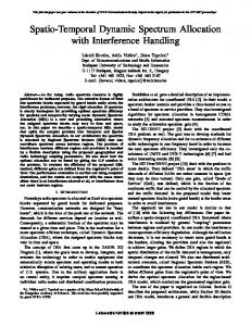
(8) This method is robust because the reduced rank smoothes the spectrum through simple time-domain windowing. The reduced rank used in the eigenvalue estimation reduces the computational load. In comparison, a statistical method for noise floor estimation works well but results in a large computational cost in the estimation of the noise power probability density function (pdf) across the band of interest. It is also dependent on the parameterization of the histogram bins used in the computations. The adaptive subspace based method does not suffer from these parameterization problems. Reduced rank processing is essential to the success and applicability of this method within a SASDR whose computing power may be limited. The variation in estimating the noise floor as a function of the rank of matrix R was studied for a variety of data sets and bands. Fig. 1 shows examples in the band 30 to 88MHz from data acquired during an exercise in theater. Fig. 1 (a) shows the computational cost of the reduced-rank methods in number of floating point operations for an 8K FFT size. Fig. 1 (b) shows the variation in the sensor noise floor estimate in dBm for various rank of the matrix R. For comparison. Fig. 1(c) shows the statistical measure of the noise floor for the same case as

Figure 1. (a) Computational cost of FLOPS vs. Rank of the reduced rank adaptive noise level estimation. (b) Noise floor variations as a function of the rank of the auto-correlation matrix R used in the adaptive noise level estimation algorithms. (c) Statistical estimation of the noise floor in dB obtained through a statistical method using histograms; the y axis represents the count number for each bin of power in dBm/Hz.

obtained by a statistical histogram computed over the band of interest. The red horizontal line in Fig. 1 (a) represents the computational cost for estimating the histogram in Fig. 1 (c). The computation cost of the subspace method shown with the blue line reduces drastically as the rank of Rl is reduces. As the rank diminishes to less than seven, some of the signal subspace starts leaking into the noise subspace. This smearing results in a slightly biased estimate of the noise floor. Robust estimations are achieved with rank 8 (within 0.5dB of the statistical measure). C. Adaptive CFAR Algorithm Once the noise floor is estimated a CFAR threshold is computed to study the spectrum occupancy and its statistics over an extended period of time (tens of seconds). To compute the CFAR threshold we use an iterative algorithm that adapts the threshold based on the number of non-coherent integrations at the fast time scale (i.e., the number of fast FFT bin power averages used to estimate spectrum occupancy) to match the noise probability density function. For a single look the CFAR is based on the averaged Rayleigh distribution of the noise floor at the sensor. For a single look the CFAR threshold is given by:

(9)

As the number of looks increases, the averaging of the noise process converges to a Gaussian distribution under the central limit theorem [13]. Multiple look averaging for noncoherent integration improves the probability of detecting signals in noise while limiting false alarms as seen in Fig. 2. After a sufficient number of fast time averages of the FFT bins, the noise statistics follows a Gaussian distribution. Using the central limit theorem approximation the threshold is then set using the inverse of the complementary error function erfc. For example a PFA of 10-4 requires a threshold of ~2.8 for a normal distribution. Using this threshold based on Gaussian statistics, a CFAR estimation is performed and the probability of detection (PD) can be computed with respect to the SNR for varying numbers of non-coherent integrations. An example of such computation is shown in Fig. 2 for a 10-4 CFAR. In Fig. 2, the red dot indicates that with only 16 noncoherent integrations, a detection probability of 0.94 is possible with a false alarm rate of 10-4 for signals only 3 dB above the noise floor. For this example a 20 MHz spectrum was measured in approximately 640 ms when averaging 16 looks (includes the time for performing the FFT on the sensor DSP). Fast time averaging helps improve the performance of the detector. Note that this improvement stems from the fact that the standard deviation around the mean of the noise’s energy level is reduced by the square root of the number of averages [14] through the simple non-coherent integration process of the Rayleigh distributed noise amplitude. The assumption is that during the fast time averaging process, the signal is stationary. This example demonstrates that a non-coherent detection algorithm can reliably detect low SNR signals through noncoherent integration and how a cost effective non-coherent detection approach can be used for the history monitoring process to provide a first cut sensing of the local spectrum usage.

IV. ESTIMATING THE STABILITY OF OPEN SPECTRUM Once the adaptive threshold is selected for the band of interest, a suite of algorithms was designed to provide an awareness of bandwidth usage to select the least used and most stable and predictable bands first. This second level of analysis is performed by the SASDR over time scales of 10s of seconds as a background task, while the network is in operation. In this process the SASDR always keeps and monitors the stability of several backup frequency bands while operating in the network. The goal of stable spectrum sensing is to provide the best quality frequency bands for opportunistic usage to maximize persistence of allocations. Persistence in spectrum allocations is key to the stability of the overall SASDR system. It reduces overhead cost of our distributed and dynamic spectrum allocation system by reducing the risk for future spectrum thrashing and the need for subsequent additional spectrum negotiation among SASDRs. The ranking of unused and stable spectrum is therefore based on a combination measure of occupancy and entropy of detectable transmissions from primary users. A. Occupancy: Based on the thresholded data, the SASDR records the amount of time a band is used over threshold. The occupancy is evaluated over a finite time window (tens of seconds) to impart confidence in determining how often a portion of spectrum contains detectable energy. Fig. 3 illustrates an example of occupancy derived from a binary map in the band 420-460MHz and measured in the suburbs of Philadelphia, PA around 11:00 a.m. in November 2004. This band contains the radiolocation/ amateur, and land mobile band (active dynamic band in urban areas). The binary map is obtained using the following equation:

(10) th

and the occupancy vector for the m frequency bin is simply given by:

(11)

Figure 2. Receiver Operating Characteristic curve showing that with fast time averaging a non-coherent detection algorithm can reliably identify signals only slightly above the noise floor while maintaining a low false alarm rate.

Figure 3. Binary map of spectrum occupancy over slow time (~30secs) in the band 420-460MHz and the occupancy vector obtained from it.

B. Entropy: The entropy statistic is the quantification of the unpredictability of a signal [8]—in this case, the aggregate transmissions of the primary radio network in the band of interest. For every frequency bin of interest the entropy measure (based on a post-threshold binary measure) is obtained as follows: First we retain in memory the spectral bin activity post threshold (binary value as seen in Fig. 3) to estimate the pdf of the time-on and time-off processes, over time (3 to 30 secs) using histograms. The transition processes in each frequency are tracked based on the differential over slow time of the binary map as defined by:

(12) K is the number of events recorded in the column for the mth frequency bin. The processes [Tm+ , Tm− ] are the transition time from unused to used and used to unused respectively. From these sets of transition times we define the processes:

and

(13)

For each of the mth frequency bins, which represents the measures of the durations of times-on and off. These vectors of time duration are then used to compute histograms of the distribution of the times-on and times-off. At present a single histogram is used to limit the processing load by combining the two processes. Once the histogram is obtained we compute H, the entropy of the process to estimate a level of predictability of the activity in this band. As new sensor data is collected, the entropy measure is updated every 5 seconds. Update a frequency bin’s entropy, H, over time and combine it with that bin’s occupancy measure. The entropy is measured using the following equation for process r.

(14) The overall entropy is the sum of both the time-on and time-off entropies, and characterizes how predictable the on/off process of spectrum usage is in these bins. Fig. 4 shows

Figure 4. 30-second map of land mobile activity, illustrating the various levels of occupancy and entropy (predictability) in bandwidth usage. The binary map is shown on top, histograms of each time-on and off processes displayed in the center and the resulting entropy measure is shown at the bottom.

examples of entropy measures and histograms used to compute such entropies from the binary map. Note that the level of entropy is related to the kurtosis of the distributions and that wide distributions (as seen in the middle histogram intensity map) have large entropy while processes with peaky distributions show lower level of entropy hence more predictability. For example a low-level entropy process is seen at approximately 454MHz and a no-entropy one at 453.45MHz with low occupancy and one with high occupancy at 452.1MHz, while large entropy processes are seen at 452.68MHz. V.

HARVESTING UNUSED/UNDER-USED SPECTRUM

The adaptive measures of occupancy and entropy discussed in Section IV are combined into a cost function using parameterized weights specified through policy as follows:

(15) The cost function is defined by setting a threshold above which the band is considered unusable and below which it is a potential band for opportunistic usage by the SASDR. Among these potential bands, the cost function is used by the spectrumallocation algorithms in order to locate and assign the most stable unused RF frequencies. Fig. 5 illustrates an example of how the combination of the two metrics is used from the binary map in the band 420-460MHz seen in Fig. 3 and measured in the suburbs of Philadelphia, PA around 11:00 a.m. in November 2004.

that spatial diversity from the network is used to limit the risk of interference. With a method for identifying the most stable spectrum resources, the network tempo can be sustained with infrequent but rapid switches to backup frequency bands that are constantly monitored across the network. What is important to notice is that some bands show very low occupancy (