Near-Optimal Dynamic Spectrum Allocation in Cellular Networks

1

Near-Optimal Dynamic Spectrum Allocation in Cellular Networks Anand Prabhu Subramanian1 , Mahmoud Al-Ayyoub1 , Himanshu Gupta1 , Samir R. Das1 , Milind M. Buddhikot2 1 Stony Brook University, NY, U.S.A. 2 Alcatel-Lucent Bell Labs {anandps, ayyoub, samir, hgupta}@cs.sunysb.edu, [email protected]

Abstract—In this paper, we address the spectrum allocation problem in cellular networks under the coordinated dynamic spectrum access (CDSA) model. In this model, a centralized spectrum broker owns a part of the spectrum and issues dynamic spectrum leases to competing base stations in the region it controls. We consider a dynamic auction based approach where the base stations bid for channels depending on their demands. The broker allocates channels to them with an objective to maximize the overall revenue generated subject to wireless interference in the network. This problem is known to be NP-hard and has been addressed before in limited context. We address this problem in a very generic context where (i) interference in the network is modeled using pairwise and physical interference models and (ii) base stations can bid for heterogeneous channels of different width using generic bidding functions. We propose efficient approximation algorithms that give near-optimal solutions with provable analytical bounds. Detailed simulation studies using randomly generated and real base station networks show that our algorithms scale very well for large network sizes.

I. Introduction Usage of wireless spectrum by radio communication devices has long been governed by governmental regulatory authorities (e.g., FCC in USA or Ofcom in UK) that divide the spectrum into fixed size chunks to be used strictly for specific purposes, such as broadcast radio/TV, cellular/PCS services, wireless LAN/PANs, public safety related communication, etc. This allocation is very long-term and space-time invariant, and is often based on peak usage per provider. Many recent observations have shown that such long-term static allocation of spectrum introduces significant inefficiencies in utilization [1]. To improve spectrum utilization, there is a new policy trend [2] to make spectrum allocation more dynamic in both spatial and temporal dimensions and more responsive to end-user demands. There can be several different architectures for providing dynamic spectrum access (DSA) that can widely vary depending on the technological limitation and usage models. For example, one can consider a very flexible architecture (like in [3]) where individual nodes are envisioned to operate over a very wide band of spectrum (e.g., 0-3 GHz range). They can perform rapid spectrum sensing to identify spectrum holes and access This work was partially supported by NSF grants CNS-0831791, CNS0721665, CNS-0721455, CNS-0721701, IIS-0713186, CNS-0519734 and CNS-0423460. Milind M. Buddhikot was partially supported by the NSF grant CNS-0435348.

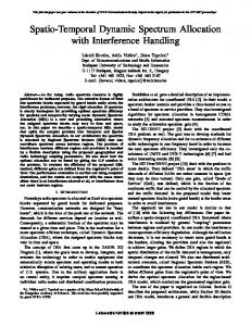
Fig. 1.

Coordinated dynamic spectrum access architecture.

the free spectrum using a completely distributed coordination mechanism. This form of DSA (often referred to as cognitive radio) may be suitable for ad hoc on-demand networks, but unnecessarily complex for infrastructure based networks, such as the commercial cellular networks used by millions of endusers worldwide. Buddhikot et al. [1], explored the application of a centralized architecture for dynamic spectrum access in cellular networks by introducing the coordinated dynamic spectrum access (CDSA) model which is much simpler and practical compared to fully distributed architectures. In the CDSA model (see Figure 1), there is a centralized entity known as the spectrum broker who owns a part of the spectrum called the coordinated access band (CAB) and dynamically allocates them to base stations in the region it controls. Indeed, centralized architectures [4–6] for dynamic spectrum access have gained a lot of interest in the research community due to their practicality and potential impact. However, success of the CDSA model hinges on the design of scalable and efficient spectrum brokers. We address this issue in this paper by designing efficient spectrum allocation algorithms that deliver near-optimal solutions. Problem Addressed. We consider a dynamic auction based approach to allocate spectrum to competing base stations. The centralized spectrum broker acts as the seller and the base stations (in the region controlled by the broker) act as the buyers of the CAB. The spectrum broker divides the CAB into channels (contiguous or non-contiguous blocks of frequency) and the base stations bid for these channels based on their spectrum demands. The base stations express their bids using a bidding function that specifies the price they are willing

2

to pay for a given set of allocated channels. Periodically, the spectrum broker allocates available channels to the base stations (based on the received bids) under the “wireless interference constraint” such that the total revenue (total price paid by the base stations)1 is maximized. The above auction based approach allows the base stations to bid according to the spectrum demands, and the spectrum broker to maximize the revenue generated from allocation of spectrum. The above spectrum allocation problem is known to be NP-hard and has been addressed before [5, 6] in limited contexts; e.g., [5] assumes unit-disk graphs to model interference between base stations, piece-wise linear bidding functions, and homogeneous set of non-overlapping channels, while [6] considers very primitive forms of bids and interference models. In contrast, we consider general network graphs and interference models (pairwise and physical), overlapping channels, and arbitrary non-complementary2 bidding functions. For the above general context, we present approximation algorithms that deliver allocations with near-optimal revenue. Ours is the first work to address the above spectrum allocation problem in such general contexts. Paper Organization: The rest of the paper is organized as follows. In Section II, we describe the system architecture of the CDSA model and give details of its components. In Section III and IV, we formally define and present efficient approximation algorithms for the spectrum allocation problem under pairwise and physical interference models, respectively. In Section V, we present detailed simulation results comparing performance of the proposed algorithms. In section VI, we discuss related work. Section VII concludes the paper with details about our future work. II. System Architecture In this section, we describe the reference system architecture (Figure 1) of our coordinated dynamic spectrum access model and give details of each important component of the model. A. Spectrum Broker (Seller) In the CDSA model, a centralized entity called the spectrum broker [1, 7] owns and coordinates access to the CAB in a given region and assigns short term spectrum leases to competing wireless service providers. Regulatory authorities like FCC can conduct one-time or long-term periodic auctions to give spectrum licenses to the broker on a regional basis. However, in contrast to existing cellular spectrum licenses, the spectrum broker can in turn grant spectrum leases that are for small geographical regions (e.g., per base station) and valid for short durations (e.g., tens of minutes) [7]. Such a spectrum lease gives the lessee exclusive rights to use the spectrum in 1 In our mechanism, bidders are charged a payment of equal amount to their bids, which maximizes the revenue without having negative utilities for bidders. Such a payment scheme may lead to “untruthful” bidding, but we ignore this aspect in this work (i.e., our auction mechanism does not try to enforce truthfulness). 2 A bidding function is said to be non-complementary when it is defined on a set of items that do not complement each other. For example, the bid for choosing two items together should not be more than the sum of the bids for choosing the items individually.

the designated region for the duration of the lease without exceeding the maximum power limit. In this paper, we mainly address the challenge of how to assign these dynamic spectrum leases to various service providers and design fast and scalable spectrum allocation algorithms. B. Base Stations or Nodes (Buyers) The region under the control of the spectrum broker can be as large as a single state having a large number (up to hundreds or even thousands) of base stations (also referred to as nodes in this article). These base stations are owned by different Radio Infrastructure Providers (RIP). The Wireless Service Providers (WSP) (e.g., AT&T, Verizon) are customers of the RIPs and use their infrastructure to provide wireless services like voice, data etc. to end-users. Each base station in the region can be used to operate different types of networks by the WSPs. For example, some base stations can be used to operate a GSM network, some for a CDMA or WCDMA network, and some for a WiMAX network. In a more general model, multiple types of networks can be operated on the same base station. Interference between different base stations depends on the location of the base stations, the frequency band used and the terrain propagation model [8]. We assume3 that the spectrum broker is aware of all the details of each base station in its region ranging from their exact location, and other characteristics like frequency range of operations, power levels, number of transmitters etc. It also knows the terrain propagation model in the region and can estimate the level of interference between base stations given their location and transmission power used. This knowledge forms part of essential inputs to our spectrum allocation algorithm. C. Coordinated Access Band (Items Sold) The portions of the spectrum that are highly underutilized or unused in spatial or temporal dimension qualify as prime candidates to be used as CAB. At the current time, good examples are Specialized Mobile Radio (SMR) (851-854/806809 MHz, 861-866/816-821 MHz), public safety bands (PSB) (764-776, 794-806 MHz), and unused broadcast UHF TV channels (450-470 MHz,470-512 MHz (channels 14-20), 512698 MHz (channels 21-51), 698-806 MHz (channels 5269)). The CAB spectrum is to be shared between different cellular services with macro-cellular infrastructures. Some of the current technology examples that can use the above CAB spectrum are 1xRTT/1xEV-DO that use 1.25 MHz channels, GSM networks that use 200KHz channels, IS-136 legacy TDMA that uses 30 KHz channels, W-CDMA networks that use 5 MHz channels, WiMAX networks that can use 1.75 MHz to 20 MHz channels. Note that different technologies often provide different forms of services. Spectrum sharing between different services is advantageous as they provide the 3 As discussed in earlier work by Buddhikot et al. [1], in this brokering model, the service providers or operators of radio access network interested in obtaining the spectrum, register with the broker and provide information on the transmitter location, capabilities (such as frequency, power, number of interfaces, preferred waveforms supported (as in CDMA, OFDM etc.)). This registration happens via a spectrum-leasing protocol that must be run on the base stations and the broker.

3

linear. The time complexity of our allocation algorithms is polynomial in the size of the bidding function. E. Auction Setting Fig. 2.

Channels of different types (widths) in the CAB.

benefit of statistical multiplexing – the services use spectrum differently and have different load factors that vary largely on a spatio-temporal scale. It is also reasonable to use existing cellular bands (450 Mhz, 800 MHz or the 1.9 GHz band) as part of the CAB, giving a guaranteed access to incumbent WSPs who already hold licenses and on-demand access to other WSPs that do not conflict with the license holders. As can be realized from the above numbers, the CAB spectrum might include hundreds or thousands of channels. Since different types of networks use channels of different widths, the spectrum broker has to make the decision on how to divide the available spectrum into channels of different widths and allocate them to different base stations. In our model, we consider the spectrum broker divides the available spectrum into some finite number of channels for each type of network. This channelization can be quite general. For example, the spectrum broker may decide to create channels of varying width as shown in Figure 2; here, if W is the total width of CAB, then for ith network/type, W/wi nonoverlapping channels of width wi are created. Note that channels of different types that overlap with each other, cannot be assigned to the same or interfering base stations. Overlapping of channels makes the spectrum allocation problem very challenging compared to only using homogeneous channels as assumed in prior work [5, 6, 9]. D. Spectrum Demands, Bids, and Bidding Functions The WSPs aggregate end-user demands at each of the base station it operates and generate spectrum demands to the broker. Spectrum demand aggregation at each base station can be done using a predictive model based on historical traffic measurements or from end-users’ bandwidth inputs. The above demands are then used to generate bids for various combination of number of channels and channel types. In general, the bids are specified using a bidding function, which may be different for different base stations. Basically, the bidding function for any base station specifies the price the base station is willing to pay for each set of channels C.4 In general, the complexity of such a bidding function can be exponential in the number of channels, since the number of possible sets of channels is exponential. However, in simpler contexts, each base station may have a separate bidding function for each channel type, and the bidding function may specify a price depending on the number of channels of that type. In this article, we do not make any assumptions about the complexity of the bidding function,5 unlike [5] where the authors assume the bidding functions to be piece-wise 4 Our

allocation algorithm does not enforce bidders to bid “truthfully.” we do assume the bidding function to be non-complementary, to prove the performance guarantee of our designed algorithms. 5 Later,

Our model corresponds to the sealed first-bid auctions, where the auctioned items are the channels. At the beginning of each allocation period, the bidders (base stations) submit their private bidding functions to the broker who chooses the “winners” based on the submitted bids. The winners are selected in a way that there is no interference (as defined later), and the total revenue (sum of bids) is maximized. III. Spectrum Allocation under Pairwise Interference In this section, we address the spectrum allocation problem under the pairwise interference model. To give a formal definition of the problem, we need to define a few terms. Later, we design a greedy algorithm, and prove that it delivers a nearoptimal spectrum allocation. We use the term node to refer to a base station. Interfering Nodes, and Interference Graph (Gt ). We now define the notion of interfering nodes in the pairwise interference model and use to define the interference graph. Definition 1: (Interfering Nodes). Two nodes are said to interfere if their corresponding “cells” (the surrounding regions they “cover” or are responsible for) intersect. Note that two interfering nodes should not be allocated the same channel for successful reception at a client located in the intersection region of their corresponding cells. Definition 2: (Interference Graph Gt .) The interference graph Gt = (Vt , Et ) is an undirected graph where each vertex represents a node and there is an edge (u, v) ∈ Et between u and v if the corresponding nodes “interfere”. Channel Graph (Gc ). The overlapping nature of the channels in the CAB is modeled using a channel graph Gc defined below. Definition 3: (Channel Graph Gc .) A channel graph Gc = (Vc , Ec ) is an undirected graph over channels as vertices, and there is an edge (ci , cj ) between two channels ci and cj if they overlap with each other. For example, the channel graph corresponding to Figure 2 will have an edge between c23 and c15 . An empty (with no edges) channel graph means that the set of channels are mutually non-overlapping (as in the model of [5]). Valid Spectrum Allocation. Informally, our spectrum allocation problem is to allocate channels to nodes so as to maximize the total revenue (total price paid by the nodes). However, the allocation of channels should be done without violating the interference constraints. We formalize the above by defining a concept of valid spectrum allocation, in terms of conflicting node-channel pairs. Definition 4: (Conflicting node-channel pairs.) Consider two node-channel pairs (u, ci ) and (v, cj ) where u and v are nodes and ci and cj are channels. The node-channel pairs (u, ci ) and (v, cj ) are said to be conflicting if the following is true: (i) u = v, or (u, v) is an edge in the interference graph, and (ii) ci = cj , or (ci , cj ) ∈ Ec (i.e., ci and cj overlap).

4

Definition 5: ((Valid) Spectrum Allocation.) A spectrum allocation is a set of allocated node-channel pairs, i.e., a spectrum allocation is a set {(u, ci )|u is a node, ci is a channel}, where a pair (u, ci ) signifies that channel ci has been allocated to the node u. A spectrum allocation I is considered valid if no two nodechannel pairs in I are conflicting. Bidding Functions and Revenue. In general, a bidding function for a node u gives the price that u is willing to pay for a set of mutually non-overlapping channels.6 For the sake of simplicity, we use an equivalent notion of total revenue generated by a given valid spectrum allocation. Below, we formally define both the terms bidding functions and revenue. Definition 6: (Bidding Function.) A bidding function Fu for a node u is a function Fu : P (C) 7→ R, where P (C) is the power set of all channels C and R is the set of real numbers. Definition 7: (Revenue R(I)). Given the bidding functions of nodes, the revenue generated by a valid spectrum allocation I is denoted by R(I) and is defined as the sum of the bids of the nodes for the channels allocated to them by the spectrum allocation I. More formally, X R(I) = Fu (Cu ), u∈Vt

where Fu is the bidding function of u, and Cu = {ci |(u, ci ) ∈ I} is the set of channels allocated to u by I. Revenue is defined only for valid spectrum allocations. In the above definition, we have implicitly enforced that the nodes are asked to pay what they bid; this could lead to “untruthful” behavior, but (as stated before) we do not enforce truthfulness in our work. Spectrum Allocation Problem. Based on the above definitions of valid spectrum allocation and revenue, the spectrum allocation problem under the pairwise interference model can be defined as follows. Definition 8: (Spectrum Allocation Problem.) Given an interference graph, a channel graph, and the bidding functions for nodes, the spectrum allocation problem is to find a valid spectrum allocation I that maximizes the total revenue R(I). Greedy Algorithm (GA). For the above spectrum allocation problem, we design a greedy algorithm that constructs a valid spectrum allocation by iteratively adding the “best” nodechannel pair at each stage. We will show that such a greedy strategy results in a valid spectrum allocation with nearoptimal revenue. A more formal description of our Greedy Algorithm for the spectrum allocation problem is as follows. Let I be the valid spectrum allocation being constructed by the algorithm. Initially, I = φ. In each iteration, the algorithm picks a node-channel pair (u, ci ) to add to I such that • I ∪ (u, ci ) remains a valid spectrum allocation, and • R(I ∪ {(u, ci )}) − R(I), the “incremental revenue” is maximum (among all choices of node-channel pairs). 6 In

this work, we do not address the problem of enforcing truthfulness.

The algorithm terminates when I cannot be extended any further. If nt is the number of nodes, nc is the number of channels, and ∆t and ∆c are the maximum vertex-degree in the interference and channel graphs respectively, then the overall time complexity of the above algorithm can be shown to be bounded by O(nt nc ∆t ∆c log(nt nc )) if we use a heap data structure to compute the maximum at each stage. Performance Guarantee of GA. In the following theorem, we will show that the Greedy Algorithm returns a nearoptimal valid spectrum allocation. However, to prove the approximation bound, we need to assume a certain “noncomplementary” property of the revenue function. Given the bidding functions, we say that the revenue satisfies the noncomplementary property if the following condition holds for any two valid spectrum allocations I1 and I2 such that I1 ∪ I2 is also a valid spectrum allocation. max(R(I1 ), R(I2 )) ≤ R(I1 ∪ I2 ) ≤ R(I1 ) + R(I2 ).

(1)

Recall that revenue is only defined for valid spectrum allocations. It is easy to see that revenue is non-complementary if and only if the bidding functions are non-complementary. The above non-complementary property is commonly assumed in the auction literature [10], and signifies that no two valid spectrum allocations “complement” one another. More importantly, the above property entails that the incremental revenue of any particular node-channel pair never increases as the Greedy Algorithm progresses (i.e., with the selection of other nodeschannel pairs). Such a property is indeed essential for the Greedy Algorithm to have a bounded performance guarantee. Later in this section, we discuss scenarios where the noncomplementary property may not be satisfied, but the Greedy Algorithm can still be modified appropriately to preserve the performance guarantee. We now prove that the revenue generated by the Greedy Algorithm is at least 1/(δt (∆c + 1) + 1) of the optimal revenue, for non-complementary revenue functions. Theorem 1: For a non-complementary revenue function, the above Greedy Algorithm (GA) returns a (δt (∆c + 1) + 1)approximate valid spectrum allocation. Here, δt is the size of the maximum independent set in the neighborhood of any node in the interference graph, and ∆c is the maximum degree of a vertex in the channel graph. Proof: Let qi be the ith node-channel pair selected by GA in its ith iteration, ai be the corresponding incremental revenue of qi , and m be the total number of iterations of GA for the given input. We use Ii to denote {q1 , q2 , ..., qi }; thus, ai = R(Ii ) − R(Ii−1 ). Let O be the optimal solution and let Om be the set of node-channel pairs in O that conflict with some pair in Im . Below, we use the notation R(I1 |I2 ) to denote R(I1 ∪ I2 ) − R(I2 ) where I1 , I2 and I1 ∪ I2 are all some valid spectrum allocations. We make the following three claims. • For each o ∈ Om , let f (o) be the smallest integer such that o conflict with qf (o) . Informally, selection of qf (o) by GA is the reason why o is not considered by GA for selection in later iterations. Note, by the greedy choice

5

of ql we have, R({o}|If (o)−1 )≤af (o) . •

By definition of δt (the maximum size of an independent set in the neighborhood of any node in the interference graph), it is easy to see that the maximum number of mutually non-conflicting node-channel pairs that conflict with a particular qi is δt (∆c + 1). Here, ∆c is the maximum degree of any vertex in the channel graph. Thus for any integer l, there are at most δt (∆c +1) nodechannel pairs o in Om such that f (o) = l. Thus we have, X

af (o) ≤ δt (∆c +1)

o∈Om •

(2)

m X

al = δt (∆c +1)R(Im ). (3)

l=1

Using induction on m, we will later show that: X R(O) ≤ R((O−Om )∪Im )+ R({o}|If (o)−1 ). (4) o∈Om

Without loss of generality, assume that the Greedy and optimal solutions are disjoint. Then, GA continues till Om = O. For Om = O, the above Equation 4 becomes: X R(O) ≤ R(Im ) + R({o}|If (o)−1 ). (5) o∈Om

Now using Equations 2 and 3 in the above Equation 5, we get R(O) ≤ (δt (∆c + 1) + 1)R(Im ), yielding the approximation ratio. Proof of Equation 4. We use induction on m. For m = 0, the equation is trivially true since I0 = {}, O0 = {}. By inductive hypothesis, let us assume Equation 4 to be true for m = l. Thus, we have X R(O) ≤ R((O − Ol ) ∪ Il ) + R({o}|If (o)−1 ). (6) o∈Ol

As before, let Il+1 = Il ∪ {ql+1 }. Since, Ol+1 is defined as the set of node-channel pairs in O that conflict with some pair in Il+1 , there are two cases: • ql+1 doesn’t conflict with any pair in (O − Ol ). Then, Ol+1 = Ol , and Equation 4 holds since R((O − Ol ) ∪ Il ) ≤ R((O − Ol+1 ) ∪ Il+1 ). ql+1 conflicts with some node-channel pairs in (O − Ol ); let O0 be the set of such conflicting pairs in (O − Ol ). Thus, we have Ol+1 = Ol ∪ O0 , where O0 ⊆ (O − Ol ). We prove induction for this case in detail below. Consider the second case above. We have, •

R((O − Ol ) ∪ Il ) =

R((O − Ol+1 ) ∪ Il ∪ O0 )

= ≤

R((O − Ol+1 ) ∪ Il ) + R(O0 |(O − Ol+1 ) ∪ Il ) (7) R((O − Ol+1 ) ∪ Il ) + R(O0 |Il )

≤

R((O − Ol+1 ) ∪ Il+1 ) + R(O0 |Il ) X R((O − Ol+1 ) ∪ Il+1 ) + R({o}|Il ). 0 o∈O

≤

(8)

Above, Equation 7 is true since R(I1 ∪I2 ) = R(I1 )+R(I2 |I1 ) for any valid allocation I1 ∪ I2 . Now, for each o ∈ O0 , let f(o) be as defined before, i.e., the smallest integer such that o conflicts with qf (o) . Since, elements in O0 do not conflict with any pair in Il , we have that: ∀ o ∈ O0 , f (o) = l + 1. Now, applying the above to Equation 8, we get X R({o}|If (o)−1 ). R((O−Ol )∪Il ) ≤ R((O−Ol+1 )∪Il+1 )+ 0 o∈O Using the above in the inductive hypothesis (Equation 6) and noting that Ol+1 = Ol ∪ O0 , we get X R({o}|If (o)−1 ), R(O) ≤ R((O − Ol+1 ) ∪ Il+1 ) + o∈Ol+1

which proves the inductive step. Thus, Equation 4 holds. It should be noted here that the bound of the above theorem is tight, which can be easily seen in simple scenarios like the one mentioned in the second remark below. Remarks. We make the following remarks, as special cases of the above result. • If each base station has a circular cell of a fixed radius, then the interference graph is a unit-disk graph, and δt is at most 5 [11]. In that case, the approximation ratio becomes 5∆c + 6. • If we consider non-overlapping channels and a unit-disk interference graph, then the above theorem states that GA returns a 6-approximate solution. This is a direct generalization of the result in [5], for arbitrary revenue functions. • If base stations are associated with circular cells of nonuniform radii, then the interference graph is a disk-graph. For disk-graphs, we can bound δt by ((2rmax /rmin )+1)2 , where rmax and rmin are the maximum and the minimum radii respectively. The approximation-ratio for disk-graphs can be further improved as follows. We divide the interference graph into subgraphs G0 , . . . , Glog(rmax /rmin ) , where subgraph Gj contains any base station with radius in [2j , 2j+1 ), and then use our techniques on each subgraph separately. Using the result from previous paragraph, the δt in each of these subgraphs is 25. Thus, the overall approximation ratio is 25(∆c + 1) log(rmax /rmin ). Handling Complementary Bidding Functions. We have so far assumed that the revenue function satisfies the noncomplementary property (Equation 1). However, there may be scenarios where the bidding functions (and hence, the revenue function) may not satisfy the non-complementary property. In many such scenarios, our Greedy Algorithm (and similarly, the algorithms designed in next section) can be modified to ensure the approximation ratio. For instance, consider the case where a node may bid for “groups” of channels, i.e., the node is willing to pay a high price for a group of channels C but bids zero price for any of the individual channels in C. More specifically, a node may

6

pay a price of 100 units for channels 5 and 10 together, but pays nothing for either channel 5 or 10 individually. Such a bidding function is complementary. However, we can have our Greedy Algorithm handle the above case by creating superchannels corresponding to each such group of channels; we also have the set of super-channels include the singleton sets of individual channels. Then, the channel-interference graph is constructed over super-channels as vertices, and allocation is done in terms of such (node, super-channel) pairs. The modified GA, which selects a (node, super-channel) pair at each stage, still yields the same approximation ratio. In a more general scenario of “packaged bids,” a service provider (owning multiple nodes) may bid for a channel c1 at a node u1 only if a node u2 is also allocated a channel c2 . In essence, a service provider may pay certain price for a group of node-channel pairs, but none for any individual pair. For the above case, the bidding functions cannot be defined independently for each node, but must be defined for each service provider (i.e., for the group of nodes owned by it). However, the revenue function can be easily computed from such bidding functions. But, the resulting revenue function is no longer non-complementary. Fortunately, our Greedy Algorithm can still be appropriately modified (by having it allocated in terms of groups of node-channel pairs) to handle the above case, while ensuring its approximation ratio. For explicitly represented bidding functions (where a price is specified for each super-channel or package), GA still runs in time which is polynomial in the size of the input (including the representation of the bidding functions). IV. Spectrum Allocation under Physical Interference In this section, we use the physical interference model to capture interference between base stations in the network, and present two approximation algorithms for the spectrum allocation problem in this context. We start by redefining the interference model and the concept of valid spectrum allocation. Interference Model. Here, we assume that each node operates using a fixed transmission power P . In the physical interference model [12], a successful reception at a distance d from a node is possible, if the Signal to Interference plus Noise Ratio (SINR) at the receiver is greater than a threshold β. More formally, a successful reception for a node u is possible at a point p if and only if, N+

P/dα P u v∈V 0

P/dα v

≥ β,

(9)

where V 0 is the set of other nodes operating on the same (or overlapping) channel as u, dx is the distance of the point p from a node x, N is the background noise, and α is the path loss exponent based on the terrain propagation model. Communication Radius (r). The communication radius r is the maximum distance from a node u within which we want the SINR from u to be greater than β. Essentially, the above is based on the stipulation that a node’s “cell” (surrounding region covered by a node) is a circular region of radius r around the node. In our context, the value of r can

be arbitrarily large (but finite), since the approximation ratio and time complexity of our designed algorithms is independent of r. Thus, the concept of communication radius must not be looked upon as an assumption. Valid Spectrum Allocation. In the context of physical interference model, a spectrum allocation I is considered valid if it satisfies the following two conditions: • For any node u, the set {ci |(u, ci ) ∈ I} of channels allocated to u consists of mutually non-overlapping channels. • For a node-channel pair (u, ci ) in I, let Vui denote the set of nodes that have been allocated in I some channel cj that overlaps with ci . More formally, let Vui = {v|(v, cj ) ∈ I and cj = ci or (ci , cj ) ∈ Ec }. Now, for I to be valid, for every (u, ci ) in I and every point p within a distance of r from u, SINR at p due to u should be greater than β; i.e, the following should hold: N+

P/dα P u v∈Vui

P/dα v

≥ β,

where dx is the distance of node x from the point p. Spectrum Allocation Problem. The spectrum allocation problem under the physical interference model is as follows. Given a set of nodes, the channel graph, and the bidding functions, the spectrum allocation problem is to select a valid spectrum allocation I that maximizes R(I), the total revenue generated by I. Distance-2 Neighbor Channels. For clarity of presentation of the algorithm description and their approximation proofs, we define the following concept. Definition 9: (Distance-2 Neighbor Channels.) Two channels are distance-2 neighbors if they are at most two hops away from each other in the channel-interference graph. In the following paragraphs, we describe two greedy algorithms, viz. GAHT and GACP, for the spectrum allocation problem under physical interference model. For both algorithms, we present worst-case guarantees on their performance depending on the interference model parameters (α and β). Our simulations results (presented in Section V) show that, in general, GACP generates higher revenue than GAHT for most values of α and β. Greedy Algorithm Based on Hexagonal Tiling (GAHT). The basic idea of GAHT is as follows. We start with partitioning the entire region into hexagonal subregions of certain length, and color them using 3 colors7 such that no two adjacent subregions have the same color. See Figure 3. Then, we construct three valid spectrum allocations, one for each color. For a particular color k, we consider only k-colored hexagonal subregions and pick node-channel pairs iteratively (as in GA). However, we impose the condition that within each hexagonal subregion, no two allocated channels are distance-2 neighbors; this condition ensures the validity of the spectrum allocation (as shown in Lemma 1). Finally, we pick the best of the three spectrum allocations (one for each color) thus 7 The coloring here is just to partition the base stations into easier-to-handle groups; it has nothing to do with channels.

7

3

2 2

2

r u

1 1 2

2 1

1

2 3

2

2 1

1 2

3

2 2

2

3

Fig. 3. Hexagonal subregions colored using three colors such that adjacent subregions have different colors. The red-colored subregions around the subregion containing node u have been partitioned into hierarchical levels; the numbers denote the hierarchical level. At lth level, there are 6l red-colored subregions.

constructed. We will prove that the above algorithm yields a near-optimal spectrum allocation (Theorem 2). Formal Description of GAHT. GAHT consists of the following steps. • Partition the entire region into hexagonal subregions of side µr each, where r is the communication radius and µ is defined as: s 2β(3α − 5) µ=4α . (10) 3(α − 1)(α − 2) Next, color the subregions using three colors, such that adjacent subregions are colored differently. See Figure 3. • For each color k, consider only the k-colored subregions and construct spectrum allocation I k as below. – Initially I k = φ. – Pick a node-channel pair (u, c) to add to I k such that the revenue of I k ∪ {(u, c)} is maximized, and I k ∪ {(u, c)} satisfies the following condition.8 In I k ∪{(u, c)}, there should be no two elements (ui , ci ) and (uj , cj ) in the same hexagonal subregion such that ci and cj are distance-2 neighbors. – Terminate when I k cannot be extended any further. 1 2 3 • From the three spectrum allocations I , I , and I thus constructed, pick the one that has the highest revenue and return it as the solution. Validity of GAHT. We now prove that each of the three •

spectrum allocations constructed by GAHT, the above algorithm, are valid. Intuitively, the spectrum allocations are valid because the total interference at any point p due to “far away” (in non-adjacent subregions) interferers is less than the signal received due to a node u in the subregion of p. Lemma 1: GAHT returns a valid spectrum allocation. Proof: Consider a node u in a subregion A of color k. As shown in Figure 3, partition all k-colored subregions surrounding A into hierarchical levels. The first level contains 6 subregions and each such subregion B is at a distance of µr from A; here, by distance between two subregions we mean 8 For sake of clarity of presentation, we have chosen this conservative condition. However, the correctness and approximation proof of GAHT is preserved even if we use the following less conservative condition: for every node-channel pair (ui , ci ) in I k ∪ {(u, c)}, there exist at most one pair (uj , cj ) ∈ I k ∪ {(u, c)} in each hexagonal subregion (including the one containing ui ) such that ci overlaps with cj . Here, uj may be equal to ui , and ci may be equal to cj .

that the distance between any point in B and any point in A is at least µr. Similarly, the√second level contains 12 subregions th at a distance of at least 2 3µr from A. In general, level √ the l 3 contains 6l subregions at a distance of at least 2 (3l − 2)µr from A. Now consider a point p within a distance of r from u. Let u be operating on a channel c. Since GAHT does not allow two elements (ui , ci ), (uj , cj ) of I k in the same hexagonal subregion such that ci and cj are distance-2 neighbors, there will be at most one node-channel pair in each k-colored hexagonal subregion that “interferes” with (u, c) in each kcolored hexagonal subregion. Thus, the total signal received at p due to all nodes possibly operating in c or an overlapping channel in the k-colored subregions other than A is at most: ∞ X l=1

6l

((

√

3 2 (3l

P − 2)µ −

1)r)α


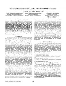
4, GACP has a better approximation ratio than GAHT. It can also be seen that the variation of the two values due to β is relatively small compared to the variation due to α. As α increases and β decreases, both GAHT and GACP become closer to the optimal performance. Revenue Comparison for Various α and β Values. We now compare the revenues generated by GAHT, GACP, and GH in a 1000 node random network and a real network (R2) with

varying values of α and β in Figure 6. Note that, in theory, increasing α means increasing the degree of deterioration in signal strength over distance traveled, which leads to more spacial reuse, and hence, higher revenue generated by all algorithms. Furthermore, decreasing β means that the receivers are less sensitive to noise and interference and are more capable of successfully receiving a transmission. This also allows for more spatial reuse, and again, higher revenue generated by all algorithms. The above patterns can be easily observed in the plots of Figure 6. As noted earlier, we see that increasing α had varying degrees of improvements in each of the three algorithms. For small values of α, GAHT and GACP generated poor and relatively similar revenues, while GH was several times better.

11 350000

350000 GAHT GACP GH

300000

300000

250000 Revenue

Revenue

250000

350000 GAHT GACP GH

200000 150000

200000 150000

150000

100000

100000

50000

50000

50000

0

0 3.0

3.5

4.0

4.5

5.0

5.5

6.0

0 2.5

3.0

3.5

4.0

α

350000

5.0

5.5

6.0

2.5

GAHT GACP GH

Revenue

150000

120000

60000

20000

0

0 6.0

0 2.5

3.0

α

(d) Real Networks, β = 1 dB Fig. 6.

GAHT GACP GH

60000 40000

5.5

6.0

80000

20000

5.0

5.5

100000

80000

50000

4.5

5.0

140000 GAHT GACP GH

40000

4.0

4.5

140000

100000

3.5

4.0

(c) Random Networks, β = 15 dB

100000

200000

3.0

3.5

(b) Random Networks, β = 7.5 dB

120000

250000

2.5

3.0

α

Revenue

300000

4.5 α

(a) Random Networks, β = 1 dB

Revenue

200000

100000

2.5

GAHT GACP GH

250000 Revenue

300000

3.5

4.0

4.5

5.0

5.5

6.0

α

(e) Real Networks, β = 7.5 dB

2.5

3.0

3.5

4.0

4.5

5.0

5.5

6.0

α

(f) Real Networks, β = 15 dB

Comparison of overall revenue generated by GAHT, GACP and GH algorithms for varying α and β values.

As α was increased, GACP’s performance greatly improved and became close to the performance of GH. B. Using GA for Physical Interference Model In this section, we modify GA (originally defined for the pair-wise interference model) to work in the context of physical interference model, and then compare the modifiedGA with GACP and GH algorithms. Recall that in the original GA, two nodes are said to interfere if they are within a certain distance d. To tailor GA to work in the context of physical interference model, we increase the distance d, until we get a “valid” spectrum allocation (based on the conservative validity-check method used in GH). In our experiments, we vary d from 2r to 8r, where r is the communication radius. We compare the revenue of a valid spectrum allocation returned by the above modified-GA algorithm with the other two efficient algorithms for physical interference model, viz., GACP and GH. We repeat this test for different values of α for a 1000 node random network and one real network (R2). The value of β is fixed at 5 dB in all experiments. In Figure 7(a) and 7(b), we show the values of d/r compared to µ0 when the spectrum allocation obtained using GA is valid under the physical interference model. In the case of random networks, d/r is smaller than µ0 by about 53% on average. In the case of real networks, we see its is smaller by about 59% on average. Note that when d/r is same as µ0 , the revenue generated by GA and GACP should be same as both algorithms are similar. Due to the smaller value of d/r, GA can exploit much higher spatial reuse of spectrum and generate more revenue. The revenue generated by both the algorithms are shown in Figures 7(c) and 7(d). The difference between the two algorithms is higher in the case of real networks due to the larger difference between d/r and µ0 compared to the random network case. This clearly demonstrates that while

the pairwise interference model is simplistic, it can be used to generate efficient spectrum allocations (with an appropriate choice of d) which are valid in the real physical interference model. But in order to prove good theoretical properties for the spectrum allocation algorithm under the physical interference model, we need to use the definition of µ0 . We also see from Figures 7(c) and 7(d) that for small values of α, the revenues generated by GA and GH are similar and, in general, are much higher than the revenue generated by GACP. For larger values of α, the difference between GACP and GA becomes smaller. VI. Related Work Traditional auctions. Auctions have been traditionally used for efficiently allocating scarce resources [16–18]. The auctioneer can maximize his revenue by selling the goods to buyers who are willing to pay the most. At the same time, the buyers also get benefited as auctions tend to assign items to buyers who need them the most based on their valuation. Some examples where auction systems have been successfully used include energy markets [17], treasury bonds [18], and selling commercial goods online [16]. In general, the goods on sale can either be a single item [10], bundle of multiple units of single items [10, 19] or bundles of multiple units of multiitems [20, 21] and the complexity of the auction mechanisms increase in this order. The spectrum allocation problem in the CDSA model differs from traditional periodic sealed bid multi-unit auctions in the following two important aspects. First, in a conventional multiunit auction, every buyer competes with every other buyers participating in the auction. In the problem considered in this work, there is a network of base stations, and each base station competes only with other base stations with which they interfere. This increases the complexity of the auction problem significantly as the way in which the base stations interfere

12 9

9

µ’ d/r

8

µ’ d/r

8

7

7

6

6

5

5

4

4

3

3

2

2 2.5

3.0

3.5

4.0

4.5

5.0

5.5

6.0

2.5

3.0

3.5

4.0

α

(a) Random Networks, d/r Vs. µ0 , β = 5 dB

5.5

6.0

140000 GACP GA GH

120000

GACP GA GH

100000 Revenue

250000 Revenue

5.0

(b) Real Networks, d/r Vs. µ0 , β = 5 dB

350000 300000

4.5 α

200000 150000

80000 60000

100000

40000

50000

20000

0

0 2.5

3.0

3.5

4.0

4.5

5.0

5.5

6.0

α

(c) Random Networks, Revenue Comparison, β = 5 dB Fig. 7.

2.5

3.0

3.5

4.0

4.5

5.0

5.5

6.0

α

(d) Real Networks, Revenue Comparison, β = 5 dB

Comparing performance of GA, GACP, and GH algorithms.

depends on external constraints that include complexities such as radio propagation model, frequency used and transceiver design etc. While traditional multi-unit auctions can be solved optimally in polynomial time, this class of auction problems are known to be NP-hard even when specific restricted class of bidding functions [5] are used. The second major difference is the overlapping nature of channels of different types which puts an additional constraint in assigning channels to base stations. In traditional auctions, any item can be assigned to any buyer that is not true here. Spectrum allocation without revenue models. Spectrum allocation algorithms, both centralized [7, 22] and distributed [9, 23] in the context of dynamic spectrum access networks have been proposed previously without any revenue model. In these works, the authors propose algorithms to allocate spectrum to different nodes thereby optimizing one or more network properties like network interference or network capacity. All these algorithms only consider pairwise interference models and do not consider heterogeneous channels of varying widths that can overlap. In context of ad hoc networks, Yuan et al. in [24] propose centralized and distributed allocation of variable width frequency blocks to nodes in the network in a time-slotted fashion. Our work differs from theirs in two main aspects. We have a general revenue model associated with the channels and try to maximize the overall revenue while they optimize a proportionally fair throughput metric. The second difference is that we propose efficient algorithms using both pairwise and physical interference models while they use only pairwise interference model. In [25], the authors propose a

spectrum allocation algorithm intergraded with interferenceaware statistical admission control. Here also, they do not consider any revenue model and use only pairwise interference model to capture interference between access points. Revenue maximizing spectrum allocation. Two previous works that are directly related to our work are [6] and [5]. In [6], Sengupta et al. formulate the spectrum allocation problem as a modification of the knapsack problem. Here they assume a very primitive revenue model where they consider a constant price for each channel and specify spectrum demands as a fixed number of channels. The spectrum broker should either allocate all channels demanded or it cannot allocate any channel. This kind of spectrum demand is too restrictive to support efficient allocation. Also, they only consider homogeneous type of channels. In [5], Gandhi et al. propose solutions for the revenue maximizing spectrum allocation problem under pairwise interference model. Here, the authors only consider a specific class of revenue function which is piece-wise linear in nature and use only homogeneous channels. Their algorithms cannot be extended to work for any general class of revenue functions and heterogeneous types of overlapping channels as we consider here. If we consider homogeneous channels only, our approximation is still better considering the fact we can solve the problem for any general revenue function. In addition, we address the spectrum allocation problem under physical interference model. Truthful spectrum auctions. Inspired by traditional work in economics, recent papers have addressed spectrum auctions from a different perspective, namely truthfulness. In

13

truthful auction mechanisms (i.e., allocation algorithms), the winners and payments are determined in such a manner that the bidders have no incentive to lie about their valuations. For instance, [26, 27] design spectrum auction mechanisms that guarantees truthful behavior from bidders, without any guarantees on generated revenue or social-welfare (sum of the valuations of the allocated items). Similarly, [28] designs an auction mechanism that guarantees resilience to certain types of collusion among bidders, while sacrificing truthfulness as well as any performance guarantees on revenue or socialwelfare. In addition, [28]’s approach requires solving an NPhard problem optimally. As noted in [29, 30], it is not possible to enforce truthfulness and guarantee an approximate revenue, since there is no way to deal with an astronomical bidder. Thus, in this article, we focus on maximizing the generate revenue, without enforcing the truthfulness property. In our future work, we plan to design an auction mechanism that is truthful and delivers guaranteed fraction of the social-welfare. Other Works. Other works worth mentioning here include [31] where a similar problem is addressed but with the goal of throughput maximization. Another paper that uses auctions to solve a related problem is [32]. Unfortunately, their restrictive interference model prohibits the use of their ideas in our setting. Finally, a concurrent work by Goussevskaia et al. [13] used ideas similar to the ones we use in GACP to solve the problem of local broadcasting in the physical interference model. VII. Conclusion and Future Work In this paper, we proposed efficient approximation algorithms that give near-optimal solutions for the spectrum allocation problem in cellular network under the coordinated dynamic spectrum access model. We addressed the spectrum allocation problem in a very general context where (i) interference in the network is modeled using pairwise and physical interference models and (ii) base stations can bid for heterogeneous channels of different width using generic bidding functions. Ours is the first work to propose efficient solutions in such general context for this problem. For the specific case of non-overlapping channels and a unit-disk interference graph, our greedy algorithm GA returns a 6approximate solution which is a direct generalization of the results in [5] for arbitrary revenue functions. Our simulations studies show that the proposed algorithms scale very well for large network topologies. Among the two algorithms proposed for the physical interference model, we see their performance primarily depends on the interference model parameters and the appropriate algorithm can be chosen based on the actual value of α and β. We also see that the simple pairwise interference model can be used to come up with efficient spectrum allocations that are valid under the physical interference model by appropriately choosing the interference region around the base stations. As part of our future work, we plan to develop techniques to model the dynamics of real spectrum demands and bids using realistic population data and user calling patterns and study the scalability of our approaches. We also plan to address the

problem of joint power and spectrum allocation in this context. Finally, we plan to address the issue of truthful spectrum auctions. R EFERENCES [1] M. M. Buddhikot, P. Kolodzy, S. Miller, K. Ryan, and J. Evans, “DIMSUMnet: New Directions in Wireless Networking Using Coordinated Dynamic Spectrum Access,” in IEEE WoWMoM, 2005. [2] Spectrum Policy Task Force, “Spectrum Policy Task Force Report,” Federal Communications Commission ET Docket 02-135, 2002. [3] DARPA XG-Program. [Online]. Available: http://www.darpa.mil/ato/programs/xg/ [4] V. Brik, E. Rozner, S. Banerjee, and P. Bahl, “DSAP: A Protocol for Coordinated Spectrum Access,” in IEEE DySPAN, 2005. [5] S. Gandhi, C. Buragohain, L. Cao, H. Zheng, and S. Suri, “A General Framework for Clearing Auction of Wireless Spectrum,” in IEEE DySPAN, 2007. [6] S. Sengupta, M. Chatterjee, and S. Ganguly, “An economic framework for spectrum allocation and service pricing with competitive wireless service providers,” in IEEE DySPAN, 2007. [7] M. M. Buddhikot and K. Ryan, “Spectrum Management in Coordinated Dynamic Spectrum Access Based Cellular Networks,” in IEEE DySPAN, 2005. [8] D. Tse and P. Viswanath, Fundamentals of Wireless Communication. Cambridge University Press, 2005. [9] L. Cao and H. Zheng, “On the Efficiency and Complexity of Distributed Spectrum Allocation,” in CROWNCOM, 2007. [10] V. Krishna, Auction Theory. Academic Press, 2002. [11] M. V. Marathe, H. Breu, H. B. Hunt III, S. S. Ravi, and D. J. Rosenkrantz, “Simple Heuristics for Unit Disk Graphs,” Networks, vol. 25, pp. 59–68, 1995. [12] P. Gupta and P. R. Kumar, “The Capacity of Wireless Networks,” IEEE Transactions on Information Theory, vol. 46, no. 2, 2000. [13] O. Goussevskaia, T. Moscibroda, and R. Wattenhofer, “Local Broadcasting in the Physical Interference Model,” in ACM SIGACT-SIGOPT DialM-POMC, 2008. [14] A. P. Subramanian, M. Al-Ayyoub, H. Gupta, S. R. Das, and M. M. Buddhikot, “Near optimal dynamic spectrum allocation in cellular networks,” in IEEE DySPAN, 2008. [15] FCC Geographic Information Systems. [Online]. Available: http://wireless.fcc.gov/geographic/ [16] EBay, http://www.ebay.com. [17] S. Borenstein, “The Trouble with Electricity Markets: Understanding California’s Restructuring Disaster,” Journal of Economic Perspectives, vol. 16, no. 1, 2002. [18] K. Binmore and J. Swierzbinski, “Treasury auctions: Uniform or discriminatory?” Review of Economic Design, vol. 5, no. 4, December 2000. [19] EBay - Multi Unit Auctions, http://pages.ebay.com/help/buy/buyermultiple.html. [20] P. Cramton, Y. Shoham, and R. Steinberg, Combinatorial Auctions. MIT Press, 2006. [21] K. Binmore and J. Swierzbinski, “Combinatorial Auction: A Survey,” INFORMS Journal on Computing, vol. 3, 2003. [22] A. P. Subramanian, H. Gupta, S. R. Das, and M. M. Buddhikot, “Fast Spectrum Allocation in Coordinated Dynamic Spectrum Access Based Cellular Networks,” in IEEE DySPAN, 2007. [23] J. Zhao, H. Zheng, and G. Yang, “Distributed Coordination in Dynamic Spectrum Allocation Networks,” in IEEE DySPAN, 2005. [24] Y. Yuan, P. Bahl, R. Chandra, T. Moscibroda, and Y. Wu, “Allocating Dynamic Time-Spectrum Blocks in Cognitive Radio Networks,” in ACM MobiHoc, 2007. [25] L. Cao and H. Zheng, “Stable and Efficient Spectrum Access in Next Generation Dynamic Spectrum Networks,” in IEEE INFOCOM, 2008. [26] X. Zhou, S. Gandhi, S. Suri, and H. Zheng, “eBay in the sky: strategyproof wireless spectrum auctions,” in MobiCom, 2008. [27] X. Zhou and H. Zheng, “TRUST: A general framework for truthful double spectrum auctions,” in IEEE INFOCOM, 2009. [28] Y. Wu, B. Wang, K. J. R. Liu, and T. C. Clancy, “A multi-winner cognitive spectrum auction framework with collusion-resistant mechanisms,” in IEEE DySPAN, 2008. [29] A. Archer, C. Papadimitriou, K. Talwar, and E. Tardos, “An approximate truthful mechanism for combinatorial auctions with single parameter agents,” Internet Mathematics, vol. 1, no. 2, pp. 129–150, 2003. [30] A. V. Goldberg and J. D. Hartline, “Collusion-resistant mechanisms for single-parameter agents,” in SODA, 2005.

14

[31] A. El-Sherif, A. K. Sadek, and K. J. R. Liu, “On spectrum sharing in cooperative multiple access networks,” in IEEE GLOBECOM, 2008. [32] K. Yang, N. Prasad, and X. Wang, “An auction approach to resource allocation in uplink multi-cell OFDMA systems,” in IEEE GLOBECOM, 2008.

(l ! 1) ' r

l 'r

A PPENDIX 'r

Proof of Theorem 2: Proof: For sake of clarity of presentation, we define two node-channel pairs (ui , ci ) and (uj , cj ) to be conflicting if they are in the same hexagonal subregion and ci and cj are distance2 neighbors. Now, among the three different colored hexagonal subregions, let us consider the subregions colored with one color at a time. Using the same notation as in Theorem 1’s proof, we make the following two claims. • For each o ∈ Om , let f (o) be the smallest integer such that o conflicts with qf (o) . Informally, selection of qf (o) by GAHT is the reason why o is not considered by GAHT for selection in later iterations. Note, by the greedy choice of ql we have, R({o}|If (o)−1 )≤af (o) . •

af (o)

≤

q(∆2c − ∆c + 1)

o∈Om

m X

al

l=1

=

stations lying in the three different colored hexagonal subregions as I k and Ok respectively where k = 1, 2, and 3. Let OP T = O1 ∪ O2 ∪ O3 . Now we have, R(OP T ) =

q(∆2c − ∆c + 1)R(Im ).

(20)

≤

o∈Om

Without loss of generality, assume that the Greedy and optimal solutions are disjoint for the considered color. Then, GAHT continues till Om = O. For Om = O, the above Equation 21 becomes: X R(O) ≤ R(Im ) + R({o}|If (o)−1 ). (22) o∈Om

Now using Equations 19 and 20 in the above Equation 22, we get R(O) ≤ (q(∆2c − ∆c + 1) + 1)R(Im ) for color being considered. Now let us denote the set of node-channel pairs chosen by the greedy algorithm and optimal algorithm for the base

R(Ok )

(23)

(q(∆2c − ∆c + 1) + 1)

3 X

R(I k )

(24)

k=1

≤

(q(∆2c − ∆c + 1) + 1)3[ max (R(I k ))]. (25) k=1,2,3

Proof of Theorem 3: Proof: Consider an arbitrary base station u whose receivers within the communication radius r should have an SINR value at least β. We divide the area around the base station into circular annuluses of width µ0 r as shown in Figure 8. The lth annulus lies between circles of radii l · µ0 r and (l + 1) · µ0 r. Note that GACP ensures that the minimum distance between any two base stations is more than µ0 r for assigning same or overlapping channels. Thus using a packing argument, the number of base stations in the lth annulus which are at least at a distance of µ0 r apart for each other is at most ((l + 1)µ0 r +

Using similar proof technique as the one used to prove Equation 4, we can show that X R(O) ≤ R((O − Om ) ∪ Im ) + R({o}|If (o)−1 ). (21)

3 X k=1

(19)

Lemma 2 shows that there cannot be more than q nodes within each hexagonal subregion that can be assigned the same channel by any optimal algorithm. Based on the above, it is easy to see that the maximum number of node-channel pairs in the optimal set that conflict with qi is at most q(∆2c − ∆c + 1). Here, ∆c is the maximum degree of any vertex in the channel graph. Thus for any integer l, there are at most q(∆2c − ∆c + 1) node-channel pairs o in Om such that f (o) = l. Thus we have, X

Fig. 8. Circular annuluses of width µ0 r around a base station. In each annulus 0 we pack circles of radius µ2r to find the number of interfering base stations that can potentially cause interference at a receiver within the communication radius of the sender base station.

µ0 r 2 2 ) π− 0 ( µ2r )2 π

(lµ0 r −

µ0 r 2 2 ) π

= 8(2l + 1).

The maximum interference I (due to other active nodes operating at the same channel as u) at any receiver p within a distance of r (the communication radius) from u can now be bounded as: ∞ X P 2α+3 P (3α − 4) I≤ 8(2l + 1) · ≤ 0α α . 0 α ((lµ − 1)r) µ r (α − 1)(α − 2) l=1

Thus, ignoring the noise, the SINR at p is at least: P rα

(α − 1)(α − 2) 0α ≥ α+3 · µ = β. I 2 (3α − 4) This shows that the GACP algorithm returns a valid spectrum allocation in the context of physical interference model. Using a proof similar to Lemma 2’s proof, we can show that no particular channel can be assigned to more than q 0 nodes in a circle of radius µ0 r, by a valid spectrum allocation. Finally, proving the worst-case guarantees of GACP can be completed using similar proof technique as the one used in Theorem 2’s proof.