A scalable non-myopic dynamic dial-a-ride and pricing problem

A scalable non-myopic dynamic dial-a-ride and pricing problem Hamid R. Sayarshad Department of Civil Engineering, Ryerson University, Toronto, ON, Canada Joseph Y.J. Chow* Department of Civil & Urban Engineering, New York University, Brooklyn, NY, USA *Corresponding author’s email: [email protected]

Abstract Non-myopic dial-a-ride problem and other related dynamic vehicle routing problems often ignore the need for non-myopic pricing under the assumption of elastic demand, which leads to an overestimation of the benefits in level of service and resulting inefficiencies. To correct this problem, a new dynamic dial-a-ride policy is introduced, one that features non-myopic pricing based on optimal tolling of queues to fit with the multi-server queueing approximation method proposed by Hyytiä et al (2012) for large-scale systems. By including social optimal pricing, the social welfare of the resulting system outperforms the marginal pricing assumed for previous approaches over a range of test instances. In the examples tested, improvements in social welfare of the non-myopic pricing over the myopic pricing were in the 20% - 31% range. For a given demand function, we can derive the optimal fleet size to maximize social welfare. Sensitivity tests to the optimal price confirm that it leads to an optimal social welfare while the marginal pricing policy does not. A comparison of single passenger taxis to shared-taxis shows that system cost may reduce at the expense of decreased social welfare, which agrees with the results of Jung et al. (2013).

Keywords: dynamic dial a ride problem, multiserver queue, dynamic pricing, approximate dynamic programming, last mile problem, flexible transport services

Accepted for publication in Transportation Research Part B, special issue on Urban Service Networks

1

1. Introduction With the compounding effects of climate change, population growth, and urbanization, travel in societies is becoming increasingly congested, and the effects of that congestion are increasingly worse. In particular, the rise of mega-regions due to urbanization poses a new set of problems for travelers. Many neighborhoods can benefit from public transit access to other parts of the megaregion, but the cost of maintaining a consistently connected system increases disproportionately with the coverage area – what transportation planners call the “last mile problem” (Chandra and Quadrifoglio, 2013). “Flexible transport services” (Mulley and Nelson, 2009) are designed to fill in the gaps where demand is too irregular for fixed schedule services to accommodate. Some of the earliest forms of flexible transport services have been around for decades, such as the “dial-aride problem” (DARP) (Wilson et al., 1976; Jaw et al., 1986; Cordeau and Laporte, 2007) and the corresponding demand responsive transit service (Schofer et al., 2003). The dial a ride problem, a subclass of the pickup and delivery problem, is defined as the problem of picking up passengers and delivering them to their destinations under tight time restrictions in a most efficient manner. For many years, such services have been deemed economically unsustainable and require heavy subsidies. This is because of problems where customers (demand) or travel (service) times are not deterministic, which give rise to stochastic DARP. The uncertainty in such problems can be modeled in a static a priori manner (e.g. Jaillet, 1988) or in a dynamic fashion as information is revealed to the fleet of vehicles over time (e.g. Dror and Powell, 1993). However, the technologies to enable dynamic operations with seamless transfer of information between passengers, vehicles, and dispatch have been limited. As a result, hybrid solutions that combine flexible routes or schedules with fixed routes have been proposed (e.g. Hadas and Ceder, 2008; Quadrifoglio et al., 2008; Nourbakhsh and Ouyang, 2011; Alshalalfah and Shalaby, 2012). Recent advances in information and communications technologies (ICTs) and “Big Data” helped alleviate the growing problem by making alternative transportation modes more viable (Chow, 2014). Due to the availability of real time vehicle location and customer request data, it is much more feasible to implement dynamic or “on-line” vehicle allocation or routing policies in flexible transit services, e.g. Psaraftis (1980), Psaraftis (1995), Madsen et al. (1995), Cortés and Jayakrishnan (2002), Horn (2002), Jung and Jayakrishnan (2011), Agatz et al., (2011), d'Orey et al. (2012), and Hosni et al. (2014). For example, Thien (2013) and Furuhata et al. (2014) present cost-sharing mechanisms for transport systems where the fare price is a proportion of total cost, and can be implemented due to the maturity of ICTs. However, as Dror and Powell (1993) pointed out, even among dynamic optimization models there is an opportunity to make use of real time data to predict and anticipate future states. Numerous studies have since shown that “non-myopic” dynamic models that can look ahead perform better than myopic dynamic models (with some exceptions – such as when myopic models get information sufficiently in advance -- Spivey and Powell, 2004): in pickup and delivery problems (Mitrović-Minić et al., 2004), in fleet management (Godfrey and Powell, 2002), in adaptive network design problems (Chow and Regan, 2011a; Chow et al., 2011); and in facility relocation problems (Chow and Regan, 2011b). The benefit of anticipating future states is that the true cost is better estimated at a specific time so as to make more informed decisions. For example, delivering a user from point A to point B does not just imply there is a marginal cost of adding the trip A-B into the vehicle’s tour, but there is an opportunity cost due to having a resource (the vehicle) tied up during that 2

time and being reposited in a location that augments the vehicle’s level of service for future users. If each vehicle is viewed as a server, the dynamic DARP is in turn a multi-server queueing system. In fact, Hyytiä et al. (2010a,b, 2012) exploit this characteristic to approximate these opportunity costs made in vehicle allocation and routing decisions. However, a fundamental assumption present in the non-myopic dynamic DARP models causes an inefficiency that has not yet been addressed in the literature: the models assume user demand is not elastic even when it should be. This flawed assumption is illustrated in Figure 1 with a simplified supply-demand graph. The essential argument made by non-myopic modelers is that systems operating under a myopic approach assume a less efficient cost curve than the true cost curve that could be achieved with a non-myopic approach. Their conclusion is that moving to a more efficient cost curve that properly accounts for opportunity costs should lead to a cost reduction represented by B – C, resulting in the point {A,C}. However, if demand is elastic, then the optimal point is not at {A,C}, but at the point where demand meets the marginal cost curve, i.e. {F,G}. Because of presuming the demand is inelastic, the system would operate at cost C, leading to excess demand of D that requires level of service of E to sufficiently meet. Myopic marginal cost curve

COST

Non-myopic marginal cost curve B E G C Demand

A

F

D

NUMBER OF USERS

A – Myopic quantity B – Myopic level of service C – Cost assumed using the non-myopic policy under inelastic demand D – Unrealized demand due to assuming full non-myopic cost at myopic quantity E – Actual cost (and resulting inefficiency) that a non-myopic policy with fixed demand assumption would induce Fig 1. Illustration of the inefficiency present assuming inelastic demand and using myopic pricing.

The inefficiency in non-myopic dynamic routing models can be corrected by considering nonmyopic dynamic pricing simultaneously, which can allow a system to move users toward {F,G}. However, no studies have jointly considered vehicle assignment, routing, and pricing in the nonmyopic dynamic DARP. Figliozzi et al. (2007) conducted one of the few studies on non-myopic pricing in dynamic vehicle routing problems for truckload routing, examining the benefits of pricing when looking ahead even one time step (part of their example is illustrated in Sec. 2.2). We propose to incorporate non-myopic pricing into the non-myopic dynamic DARP, as Figliozzi et al. (2007) had done for truckload routing. Contrary to that earlier study, our proposed contribution is not limited to only a single time step look-ahead, but instead approximates the 3

expected average future value from an infinite horizon. This is accomplished by adopting the multi-server queue approach from Hyytiä et al. (2012) to approximate the average future value. We introduce a non-myopic pricing component from the queueing literature into the dispatch and routing policy function. The methodology is numerically illustrated for a replicable example, and then compared over a range of test instances against the myopic pricing assumption to demonstrate its effectiveness.

2. Literature review 2.1. Non-myopic dynamic dial a ride problem As mentioned, DARPs have been around for a long time. In addition to the studies cited above, heuristics to solve DARPs have been proposed by Psaraftis (1983), Jaw et al. (1986), Cordeau and Laporte (2003), Diana and Dessouky (2004), Kirchler and Calvo (2013), Paquette et al. (2013), Ma et al. (2013), and Martinez et al. (2014), among others. A comprehensive review of static or even myopic dynamic DARP variations and solution algorithms is beyond the scope of this study. There are a couple of non-myopic methods proposed in the literature for the dynamic DARP, as well as for the related dynamic pickup and delivery problems. Both are reviewed here. Berbeglia et al. (2010) classified these problems into three different classes: the dynamic vehicle routing problem with pickups and deliveries (Dynamic VRPPD), the dynamic stacker crane problem (Dynamic SCP), and in the case where the transportation requests consists of passengers the problem is the dynamic dial-a-ride problem (Dynamic DARP). While the static DARP is primarily challenging because it’s an NP-hard problem, the dynamic problem with look ahead faces a different set of challenges. A non-myopic dynamic optimization problem is solved either as an optimal control differential equation (for continuous time and decision problems) or a Markov decision process (for discrete time decision problem) of a form in Eq (1) (shown in discrete time form), called the Bellman equation (Powell, 2011). 𝑉𝑡 (𝑅𝑡 ) = min(𝐶𝑡 (𝑅𝑡 , 𝑥𝑡 ) + 𝛾𝐸[𝑉𝑡+1 (𝑅𝑡+1 )|𝑅𝑡 ]) xt

(1)

where 𝑉𝑡 is the value of the policy, 𝐶𝑡 is the immediate payoff of the decision 𝑥𝑡 under state 𝑅𝑡 (which is also typically driven by information on exogenous stochastic variables, and varies in size based on the underlying distribution of the variable(s)), and 𝛾 is a discount factor. The challenge is in determining an appropriate value for the last term, 𝐸[𝑉𝑡+1 (𝑅𝑡+1 )|𝑅𝑡 ]. The conditional expectation term depends on the future state 𝑅𝑡+1 , but 𝑅𝑡+1 depends on 𝑅𝑡 and may also depend on 𝑥𝑡 . As either of these variables increase, and as the number of discrete time steps increases, the problem quickly becomes intractable to solve. The networked variant with explicit optimal timing is shown by Chow and Regan (2011a) to be altogether unsolvable in its complete form because even when 𝑅𝑡+1 is independent of 𝑥𝑡 , there is an additional complexity due to 𝑉𝑡,𝑖 for network component 𝑖 being dependent on 𝑉𝑡−1,𝑗 for network component 𝑗. As a result, the Bellman equation becomes one that depends on both past (through network effects) and future (through expected value function), leading to no exact solution method possible. The intractable problem is shown in Eq (2), where 𝐾 is the number of link components that can be decided upon. 4

𝑉𝑡,𝑖 (𝑅𝑡 ) = min(𝐶𝑡 (𝑅𝑡 , 𝑥𝑡,𝑖 ) + (𝑉𝑡,1 (𝑅𝑡 , 𝑥𝑡,𝑖 ) + ⋯ + 𝑉𝑡,𝑖−1 (𝑅𝑡 , 𝑥𝑡,𝑖 ) + 𝑉𝑡,𝑖+1 (𝑅𝑡 , 𝑥𝑡,𝑖 ) + ⋯ xt,i

+ 𝑉𝑡,𝐾 (𝑅𝑡 , 𝑥𝑡,𝑖 ) + 𝜌𝐸[𝑉𝑡+1,𝑖 (𝑅𝑡+1 )|𝑅𝑡 ])

(2)

Chow and Regan (2011a) considered the network design and timing problem in Eq (2), and proposed an intermediate value function as a policy approximation, which can be solved with asymptotic convergence by enumerating multiple sequences ℎ ∈ 𝐻 for timing a set of network decisions. Even the intermediate function, shown in Eq (3), exhibits a greater curse of dimensionality (due to network dependencies) than the form shown in Eq (1). 𝑉𝑡,𝑖ℎ (𝑅𝑡 ) = min(𝐶𝑡 (𝑅𝑡 , 𝑥𝑡,𝑖ℎ ) + 𝑉𝑡,(𝑖+1)ℎ (𝑅𝑡 , 𝑥𝑡,𝑖ℎ ) + 𝜌𝐸[𝑉𝑡+1,𝑖ℎ (𝑅𝑡+1 )|𝑅𝑡 ])

(3a)

where 𝑉𝑡 = minh (𝑉𝑡,1ℎ )

(3b)

xt,ih

where the value of one network decision also depends on the performance of other network decisions at the same time (and approximated using minimum of a series of enumerated sequences). Due to these challenges, many have proposed approximate dynamic programming methodologies, where either one or more of the following elements are approximated: policy (Secomandi, 2001) (state dependent decision rule), value function (Thomas and White, 2004), contribution function, or state (Figliozzi et al., 2007). Researchers working with non-myopic dynamic DARP have dealt with the approximation using Markov decision processes under different structural variations. Dror at al. (1989) and Dror (1993) proposed a Markov decision model for the vehicle routing problem. These models were formulated as a multistage stochastic programming problem. Secomandi (2001) presented a version of dynamic programming model for the vehicle routing problem where customers' demands are uncertain. The objective function minimizes the expected distance traveled in order to serve all customer demands. Neuro-dynamic programming was used to provide approximate solutions to this difficult stochastic combinatorial optimization problem. Spivey & Powell (2004) proposed a generalized dynamic assignment problem for fleet management as a Markov decision process, where a resource (container, vehicle, or driver) can serve only one task at a time. Novoa and Storer (2009) presented an approximate dynamic programming algorithm for the single-vehicle routing problem with stochastic demands from a dynamic or re-optimization perspective. They extended Secomandi’s one-stage look-ahead to a two-stage look-ahead. Cortés et al. (2009) formulated the problem as a hybrid predictive control problem using state space models, also using a two-stage look-ahead, and proposed a particle swarm optimization (PSO) heuristic to solve it. Innovative approximations of future states have also been proposed. Mitrović-Minić et al. (2004) introduced a dynamic problem with two rolling horizons, one for short term and one for long term. Spivey and Powell (2004)’s policy includes the use of gradients to approximate the future values. Ichoua et al. (2006) introduced a strategy based on dummy customers (repesenting forcasted requests) in the vehicle routes to respond to future request arrivals. Chow and Regan (2011a) approximated the future states in adaptive network design problems with a Least Squares Monte Carlo simulation method that is widely used in the real option literature. This method was shown to be applicable to dynamic DARP by Chow and Sayarshad (2015). A third direction in the literature focused on alternative strategies. In addition to the dispatch strategy considered by many studies, Thomas and White (2004) formulated a dynamic 5

route selection for a single pickup and delivery as a Markov decision process that anticipates demand requests. Thomas (2007) also looked at the waiting strategy for vehicles to determine a policy for when to wait and when to reposition. Much of the dynamic programming based approaches cannot solve large scale problems without approximating very short time horizons (e.g. 1 step look ahead) or aggregated states. Hyytiä et al. (2012) proposed approximation in the service process instead, treating it as a multiserver queue to obtain analytical expressions for steady state performance that can be easily computed for large scale systems. A summary of recent contributions to non-myopic dynamic DARPs is provided in Table 1. Table 1. Summary of non-myopic dynamic DARP studies Studies Approximation features(s) Dror et al. (1989) Markov decision process framework; No solution provided Secomandi (2001) Cyclic rollout policy for value Thomas and White (2004) One-stage look-ahead Mitrović-Minić et al. (2004) Double horizon insertion heuristic Spivey and Powell (2004) Gradient approximations of value Ichoua et al. (2006) Dummy customers for state; Tabu search heuristic Thomas (2007) Five insertion heuristic policies Novoa and Storer (2009) Cyclic rollout policy for value; Monte Carlo simulation Cortés et al. (2009) Two-stage look-ahead; Particle swarm optimization Hyytiä et al. (2012) Multi-server queue for value Chow and Sayarshad (2015) Least Squares Monte Carlo method

2.2. Motivational example for non-myopic pricing These existing approximation methods have not included the pricing strategy as a non-myopic policy. The challenge with incorporating pricing in many of these problems, which are typically formulated as discrete state spaces with discrete decisions, is the continuous nature of the pricing variable. Figliozzi et al. (2007) illustrate the need for non-myopic pricing using a simple 4-node example, which we reproduce here as a DARP and expand upon with respect to the motivation. Consider a network illustrated in Figure 2, where a single vehicle fleet serves 4 nodes located around a square block. The vehicle would have to traverse to node C or node A from node B in order to reach node D. The lengths of each link is 1 unit time step, and one of two possible requests occurs each step: a customer either (a) desires to be picked up at node A to be dropped off at node B (50% probability), or (b) they wish to be picked up at node D to be dropped off at node A (50% probability). We assume no dwell times and no repositioning costs. The willingness to pay of each customer is distributed as 𝑝(1) = 0.25, 𝑝(2) = 0.50, 𝑝(3) = 0.25.

6

B

C

Lengths: |𝐴𝐵| = |𝐵𝐶| = |𝐶𝐷| = |𝐷𝐴| = 1 A

D

Fig 2. Motivational example for non-myopic pricing (adapted from Figliozzi et al., 2007).

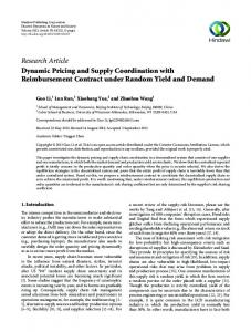
Static price: Both AB and DA have the same cost of 1 unit, so under a static pricing scheme the vehicle would charge the passengers the same cost of 1 unit. This is the pricing policy used in many taxis, for example. Myopic dynamic price: In this case, the price depends on where the vehicle is currently positioned. Suppose the vehicle is located at node A. In order to serve customer AB, the vehicle would have a cost of 1 unit. On the other hand, serving customer DA would have a cost of 2 units (A-D-A). Non-myopic dynamic price: Now let’s consider the consequence of serving customer AB from node A. After serving that customer, the vehicle would be located at node B. If a new customer arrives at AB, the cost would be 2 (B-A-B). With the distribution of the willingness to pay, the expected user benefit is (3 − 2)(0.25) = 0.25. If the new customer instead requests DA, the cost is 3 (B-C-D-A), with an expected user benefit of 0. The expected user benefit from this scenario is 0.5(0.25) + 0.5(0) = 0.125. If the vehicle is at node A because the initial AB customer turns down the service due to price, the expected user benefit of a subsequent AB is 0.5(2 − 1) + 0.25(3 − 1) = 1, while that for DA is 0.25(3 − 2) = 0.25. The expected benefit is 0.5(1) + 0.5(0.25) = 0.625. The price for the initial AB is set equal to the cost of the accepted service (1) minus expected user benefit from accepted service (0.125) plus the opportunity cost due to expected benefit from rejected service (0.625). The result is an optimal price of 1 − 0.125 + 0.625 = 1.5, which differs from the myopic dynamic price of 1 unit for AB at node A. As this example shows, not properly anticipating/looking ahead for the opportunity costs or benefits can result in suboptimal pricing. Figliozzi et al. (2007) modeled the future costs by approximating them with a single time step finite horizon. 2.3. Hyytiä et al.’s model One more recent methodology was to approximate the value function with a multi-server queue system (Hyytiä et al., 2010a, b, 2012). Their argument is that, instead of approximating short time horizons, value functions, or states, why not approximate the overall system as a queueing system? As a stochastic queueing system, it is possible to derive analytical expressions for the steady state average delay costs, which is computationally cheap. It is then possible to approximate steady state costs of an infinite horizon for a large scale problem setting, which is not even possible with the current state of the art non-myopic DARP methods. An illustration of 7

the approximation is shown in Figure 3. By assuming that request arrivals with rate λ are timeinvariant Poisson processes and approximating the server time with rate 𝜇 as Poisson processes, the steady state (assuming infinite horizon) cost to allocate a new customer to a vehicle can be determined as the change to the steady state queue delay. Whereas a non-myopic approach under a queueing system uses the steady state variables, the myopic approach simply uses the current delays observed in the queues. Veh. 1 Veh. 1

Veh. 3

Veh. 2

Veh. 3

Waiting to be served

Existing pickup Veh. 2

Being served

New arrival

New arrival λ

Existing dropoff

μ

Fig 3. Illustration of the non-myopic dynamic DARP as a multi-server queue system.

Under this approximation, both the network effects and the timing effects (as illustrated with an intermediate value function from Eq (2) are lumped together into one effect as shown in Eq (4). 𝑉𝑡,𝑖 (𝑅𝑡 ) = min (𝐶𝑡 (𝑅𝑡 , 𝑥𝑡,𝑖 ) + Ω(𝑉𝑡,1 , … , 𝑉𝑡,𝑖−1 , 𝑉𝑡,𝑖+1 , … , 𝑉𝑡,𝐾 , 𝐸[𝑉𝑡+1 |𝑅𝑡 ])) xt,i

(4)

where Ω is approximated by an expression derived from M/M/s queue and the whole expression is split into user costs and system costs, shown in Eq (5). 𝑎𝑟𝑔𝑚𝑖𝑛𝑣,𝜉 [𝑐(𝑣, 𝜉) − 𝑐(𝑣, 𝜉 ′ )]

(5a)

where 𝑐(𝑣, 𝜉) = 𝜃𝑇(𝑣, 𝜉) + (1 − 𝜃) (𝛽𝑇(𝑣, 𝜉)2 + ∑ 𝑆𝑖 (𝑣, 𝜉))

(5b)

𝑖

where 𝑣 is a vehicle, 𝜉 is a tour obtained for a traveling salesman problem with pickup and delivery (TSPPD), 𝜉 ′ is the previous tour updated to the time of the current customer arrival, 𝑐 is the value function, 𝑇 is the tour length, 𝑆𝑖 is the total delay for customer 𝑖 (service plus wait time, i.e. time from call in to time they are delivered), and 𝜃 and 𝛽 are parameters to adjust the degree of system cost versus user cost (𝜃) and degree of look ahead (𝛽). The method is shown to be easy to implement even for large systems (up to fleets of 140 vehicles) and improves upon the myopic solution for a range of parameter values. While an M/M/s approximation is not how the system truly behaves, it is empirically shown using simulation to outperform a myopic policy. We know that some form of approximation is required for such systems, whether it is a finite rolling horizon (as done by Figliozzi et al., 2007), 8

an approximation of the states, an approximation of the value functions, or otherwise, and the approximation method from Hyytiä et al. (2012) has the added benefit of computational efficiency. The method has been implemented in practice with the Kutsuplus in Helsinki (Barry, 2013). Fare prices are not discussed by Hyytiä et al., and as such are not included in the optimal policy.

2.3. Non-myopic pricing in queues Since the approximation in Hyytiä et al. (2012) is based on an M/M/1 queue, we examine the literature on tolling in queues as a means of incorporating pricing into the non-myopic policy. It has long been known (Naor, 1969) that a queue for a public good that does not impose any toll would lead to a suboptimal social value. Tolling and other strategies to assign priority to customers based on their willingness to pay are needed to attain a social optimum. While Naor (1969) made this argument for an M/M/1 queue, Knudsen (1972) also showed this for an M/M/s queue (this is also obvious from the marginal cost pricing literature for roads, as discussed in Yang and Huang, 1998). Mendelson and Whang (1990) distinguished the aggregate arrival rate from an individual decision structure of whether to join the system. In the individual decision system, there exists an actual rate of pre-arrivals Λ where individuals each have an effective arrival rate 𝜆, 0 < 𝜆 ≤ Λ, representing their expected arrival (no balking or reneging) of entering the system at the level of service that they are willing to pay. The authors derive a demand function at the individual level by first defining the probability that an arrival values the service at 𝑥 or higher as shown in Eq (6). ∞

̅ (𝑥) = 1 − Φ(𝑥) = ∫ 𝜙(𝑧)𝑑𝑧 Φ

(6)

0

where Φ(x) is the cumulative probability of willingness to pay for service 𝑥. Since the arrival ̅ (𝑥), the marginal value (willingness to pay), V ′ (λ), is the value 𝑥 rate is then 𝜆 = ΛΦ corresponding to the expression, shown in Eq (7). 𝜆 ̅ −1 ( ) V ′ (λ) = Φ Λ

(7)

Let 𝑊(𝜆) be the time spent in the system. At the equilibrium, the user would be indifferent between joining and not joining the system, resulting in Eq (8). V ′ (λ) = 𝑝 + 𝜓𝑊(𝜆)

(8)

where 𝑝 is the cost to the user, and 𝜓 is value of time faced by an incoming arrival. At the social optimum, the first order condition results in Eq (9), and combining that with Eq (8) leads to the social optimal toll 𝑝∗ shown in Eq (10). V ′ (λ∗ ) = 𝜓𝜆∗

𝑑𝑊 + 𝜓𝑊(𝜆∗ ) | 𝑑𝜆 𝜆=𝜆∗

(9)

9

p∗ = 𝜓𝜆∗

𝑑𝑊 | 𝑑𝜆 𝜆=𝜆∗

(10)

3. Proposed methodology Our approach to integrating non-myopic pricing is as different from Figliozzi et al.’s (2007) approach as Hyytiä et al.’s (2012) approach is different from the existing non-myopic dynamic DARPs that only provide one- to two-step look ahead. The precise dynamic DARP that we are solving is described below.  A fleet of vehicles receives dispatch, routing, and pricing instructions from a central authority.  Customers call in requesting service from one location to another; as a result, dispatch, routing, and pricing decisions are made in real time by the central authority. The subgraph during each dispatch assignment consists of 𝐺 = {𝑂, 𝐷, 𝑃 + , 𝑃− }, where 𝑂 is the current vehicle location, 𝐷 is a pre-specified idle vehicle destination, 𝑃+ is the set of pickup nodes, and 𝑃− is the set of drop-off nodes, where |𝑃+ | ≤ |𝑃 − | since a vehicle may be en-route to drop off a passenger when a new passenger arrives. In the numerical experiments in this study, 𝐷 is set to be the fleet depot, but in future studies we intend to call an assignment routine to preposition the idle vehicle. All vehicles at the start of the day are located at the depot, but future studies will examine the initial prepositioning problem as well. Prebooking, reservations, etc., are not explicitly handled. As noted in de Borger and Fosgerau (2012), the cost of waiting can be transferred to the cost of inconvenience in trip planning, depending on information provision.  Customers’ requests in typical DARPs include time windows for pickup and drop-off. Hyytiä et al. (2012) studied the DARP without time windows. We follow this assumption of no time windows, but justify it as being built into the elastic demand function – since the objective has user cost, the pricing would reflect late deliveries, which in turn feeds back to the demand for service.  Requests are assumed to be from single individuals arriving in a Poisson process. Group arrivals and more complex arrival processes are not modeled here; these properties can be explored in future research. Vehicles have a capacity for the case of shared use service.  Based on the price quoted by the system, a customer may choose to reject the service. As a result, user demand is elastic.  Once a vehicle is assigned to a customer, the dispatch decision and price do not change (the route sequence may change if the vehicle is assigned to subsequent arrivals). As discussed in Furuhata et al. (2014), different cost-sharing mechanisms may be possible and user behavior may be sensitive to them, but price updating as well as cost-sharing mechanisms will be considered in future research. By assuming no elasticity in the demand (i.e. fixed 𝜆 that is not based on cost of service), the non-myopic policy will over-discount the cost of service, leading to inefficiency. To correct the problem, we need to introduce the fare pricing decision variable that achieves social optimum for the steady state queue. 𝑉 ′ (𝜆) in Eq (7) to Eq (9) is an inverse demand function. The 𝑉(𝜆) is 10

𝛼

required to be strictly concave. We assume a linear demand function, 𝑉′ = 𝛼 − Λ 𝜆, such that the value function is shown in Eq (11), although other concave functions can also be used. 𝑉 = 𝛼𝜆 −

𝛼 2 𝜆 ,0 < 𝜆 ≤ 𝛬 2Λ

(11)

If we make the same M/M/1 approximation as Hyytiä et al. (2012), the average delay for a user can be defined as shown in Eq (12). 𝑊=

1 𝜇−𝜆

(12)

The parameter 𝜇 is exogenous and approximated with 𝜇̂ obtained from historical data, as is the parameter 𝛼. For the non-myopic DARP, the service time is the time a user is picked up until they are dropped off. If we call this time for user 𝑖 (from a finite population 𝑁) to be 𝑥𝑖 , then the value of 𝜇̂ is determined by Eq (13). 𝜇̂ =

1 1 ∑ 𝑁 𝑥𝑖

(13)

𝑖

Taking the derivative of 𝑊 with respect to 𝜆, we get: 𝑑𝑊 1 = (𝜇 − 𝜆)2 𝑑𝜆 Then the social optimal fare price to charge incoming user 𝑛, considering steady state queue performance, is dependent on the social optimal 𝜆∗𝑛 as shown in Eq (14). We assume that the prices are set marginally, based on the additional cost to the tour and the user cost. This assumption will be used when computing the social welfare of this policy in the experimental study. 𝑝𝑛∗ = 𝜓𝜆∗𝑛

1 (𝜇̂ − 𝜆∗𝑛 )2

(14)

When implementing this as a dynamic DARP, the prices of all passengers that already accepted service are fixed (per our assumptions described earlier), and we only need to solve 𝜉, 𝜆, 𝑝 for each vehicle 𝑣 for the new passenger under consideration, and select the maximum value increase. If cost-sharing mechanisms are to be considered, it may be implemented here in a future study as a price updating scheme for all passengers being served by the vehicle. For each new passenger 𝑛, the optimal policy when including the price from Eq (14) is shown in Eq (15) derived from Eq (5). In Eq (15), the objective is to maximize value instead of minimizing cost, 𝛼 and the expression includes the added benefit of a single new customer (𝛼𝜆𝑛 − 2Λ 𝜆2𝑛 ) as well as

11

𝜓𝜆

the price transfer ((𝜇̂−𝜆𝑛 )2 ) in the user and system costs. We also divide the costs by 𝑇(𝑣, 𝜉𝑛 ) to 𝑛

ensure the units are the same as the benefits. max 𝑍𝑛 (𝜆𝑛 ; 𝑣, 𝜉𝑛 ) − 𝑍 ′ (𝑣, 𝜉𝑛−1 )

(15a)

where 𝜓𝜆𝑛 𝛼 2 𝜃 (𝑇(𝑣, 𝜉𝑛 ) − (𝜇̂ − 𝜆𝑛 )2 ) 𝑍𝑛 (𝜆𝑛 ; 𝑣, 𝜉𝑛 ) = 𝛼𝜆𝑛 − 𝜆 − 2Λ 𝑛 𝑇(𝑣, 𝜉𝑛 ) 𝜇̂ 𝜆𝑛 𝜓𝜆𝑛 (1 − 𝜃) ( 𝑇(𝑣, 𝜉𝑛 )2 + ∑𝑛𝑖=1 𝑆𝑖 (𝑣, 𝜉𝑛 ) + ) 2(𝜇̂ − 𝜆𝑛 ) (𝜇̂ − 𝜆𝑛 )2 − 𝑇(𝑣, 𝜉𝑛 )

(15b)

The parameter 𝜃, 0 ≤ 𝜃 ≤ 1, is a weight to differentiate user cost from system cost. To solve for 𝜆∗𝑛 , we take the derivative of 𝑍𝑛 with respect to 𝜆𝑛 and set it to zero, 𝜕𝑍𝑛 ⁄𝜕𝜆𝑛 = 0, shown in Eq (16) which can be solved with a simple one-dimensional line search. A price updating mechanism would require more sophisticated solution method over all passengers being served by the vehicle, which is avoided here. 𝛼−

𝛼 ∗ 𝜓 2𝜓𝜆∗𝑛 𝜆𝑛 + 𝜃 ( + ) Λ 𝑇(𝑣, 𝜉𝑛 )(𝜇̂ − 𝜆∗𝑛 )2 𝑇(𝑣, 𝜉𝑛 )(𝜇̂ − 𝜆∗𝑛 )3 𝜇̂ 2 𝑇(𝑣, 𝜉𝑛 ) 𝜓 2𝜓𝜆∗𝑛 − (1 − 𝜃) ( + + ) = 0, 2(𝜇̂ − 𝜆∗𝑛 )2 𝑇(𝑣, 𝜉𝑛 )(𝜇̂ − 𝜆∗𝑛 )2 𝑇(𝑣, 𝜉𝑛 )(𝜇̂ − 𝜆∗𝑛 )3

(16)

0 < 𝜆∗𝑛 ≤ Λ

In real-time operations (and for simulations of such operations), Algorithm 1 is used. Algorithm 1 Upon arrival of a new user 𝑛, 1. Update the positions and service statuses of the 𝜉𝑛−1 tours of every vehicle from the time of previous user 𝑛 − 1. 2. For each vehicle 𝑣, a. Solve a TSPPD algorithm (Algorithm 2) to obtain potential tour 𝜉𝑛 b. Determine 𝜆∗𝑛 and 𝑍𝑛 (𝜆∗𝑛 ) (the prices 𝑝𝑛∗ can also be computed using Eq (14)) 3. Pick the vehicle that maximizes Eq (15a). Update 𝜉𝑛 as the new tour for that vehicle, while keeping the other vehicles’ tours the same as before. In this optimization model, the price assigned to the new customer is a function also of (v, ξ) because the assignment and route determine the resulting 𝑥𝑖 (as a DARP, some existing customers might get reshuffled). For example, user 1 may be assigned to vehicle 1, but when user 2 arrives it might get picked up and dropped off by vehicle 1 if it’s along the way and the solution maximizes the value. As such, we acknowledge (just like Hyytiä et al.) that the M/M/1 assumption is not reflective of operating conditions since FIFO conditions are violated. The approximation is assumed to build in the steady state considerations into the policy. All prices 12

are set at an equilibrium that assumes users have just enough incentive to choose the service, so no rejections or balking actually occurs during a simulation of the dynamic policy. For the TSPPD, a heuristic is introduced based on the one discussed in Mosheiov (1994) and shown in Algorithm 2. The difference is that we are evaluating a reoptimization-based approach, where some users might have already been picked up earlier. In those cases, those users would only have a drop-off node while counting toward the initial capacity. Algorithm 2 – reoptimization-based TSPPD insertion algorithm For a given current vehicle location 𝑂, a set of pickup nodes 𝑃+ and drop-off nodes 𝑃− , a vehicle capacity 𝐾, and distances between every node pair 𝑐𝑢𝑤 , 1. Create a TSP tour 𝑆 for {𝑃− , 𝑂} 2. For each 𝑢 ∈ 𝑃+ , insert 𝑢 into 𝑆 such that a. capacity constraint at that insertion point and all subsequent nodes is feasible, b. 𝑢 is visited before its corresponding drop-off, and c. increased tour length is minimized 3. Update capacities at each node in the tour from insertion point, and go to step 2 For the experimental study in Sec. 4, the TSP tour construction of the drop off nodes in step 1 of Algorithm 2 is solved using Christofides’ (1976) algorithm. Alternative routing and insertion algorithms can certainly be substituted in (and encouraged for practitioners). While the contribution of the study is focused on evaluating the improvement of the non-myopic pricing, the Christofides’ algorithm is known to have a worst case bound of 50% of the optimal value. To ensure that the algorithm works well enough for the experimental study, the results are compared against an exact solution obtained using CPLEX on an integer programming (IP) formulation of the TSP for step 1. The IP formulation that can be used on the drop-off node tour construction is shown in Eq (17). min

∑

∑

𝑢∈{𝑃− ,𝐷}

𝑤≠𝑢, 𝑤∈{𝑃− ,𝐷}

𝑐𝑢𝑤 𝑋𝑢𝑤

(17a)

Subject to ∑ 𝑋𝑂𝑤 = 1

(17b)

𝑤∈𝑃−

∑ 𝑋𝑤𝐷 = 1

(17c)

𝑤∈𝑃−

𝑢, 𝑤 ∈ 𝑃−

𝑇𝑢 + 𝑐𝑢𝑤 − 𝑇𝑤 ≤ (1 − 𝑋𝑢𝑤 )ℳ, 𝑐𝑂𝑤 − 𝑇𝑤 ≤ (1 − 𝑋𝑂𝑤 )ℳ, 𝑋𝑢𝑤 ∈ {0,1},

𝑤 ∈ 𝑃−

𝑇𝑢 ≥ 0

(17d) (17e) (17f)

In terms of performance measures, let 𝜏1𝑛 be the realized clock arrival time of user 𝑛, 𝜏2𝑛 be the realized pickup time of user 𝑛, and 𝜏3𝑛 be the drop-off time of user 𝑛. The marginal pricing for user 𝑛 (for determining social welfare for the policy from Hyytiä et al. (2012)) is then set equal to the value shown in Eq (18). 13

𝑝𝑚𝑎𝑟𝑔𝑖𝑛𝑎𝑙,𝑛 = 𝜓[𝑇(𝑣, 𝜉𝑛 ) − 𝑇(𝑣, 𝜉𝑛′ )]

(18)

The social welfare, computed as the total value to the users minus the total costs to the users, is computed as shown in Eq (19). More specifically, for a given vehicle 𝑣 and (feasible) route 𝜉, let 𝑆𝑛 (𝑣, 𝜉𝑛 ) denote the total delay of a customer n in the system, and 𝑇(𝑣, 𝜉𝑛 ) the tour length of vehicle 𝑣 for passenger 𝑛. Thus, total costs to the users are computed by the total sojourn time and fare price of all customers divided by the current work backlog of vehicle 𝑣. 𝑝 (𝑆𝑛 (𝑣, 𝜉𝑛 ) + 𝑛 ) 𝛼 2 𝜓 𝑆𝑊 = ∑ (𝛼𝜆𝑛 − 𝜆𝑛 ) − ∑ 2Λ 𝑇(𝑣, 𝜉𝑛 ) 𝑛

(19)

𝑛

4. Experimental study The experimental study is designed to address five questions: 1) Does the proposed methodology work? This question is resolved in Sec. 4.1 with a replicable example (input parameters and outputs provided in the Appendix) and comparison between the policy from Hyytiä et al. (2012) (which we will call the marginal pricing policy) and our proposed policy that accounts for non-myopic pricing. 2) Does the assumption of TSPPD heuristic matter to the relative comparison between myopic and non-myopic policies? To answer that question, we run the same base scenario instances uing Algorithm 2 with step 1 solved separately by Christofides’ algorithm and using CPLEX to solve the IP formulation. 3) How much better does our policy work in terms of social welfare of our users? Assuming that a marginal cost policy is used when not considering non-myopic pricing, we can compute the social welfare for simulated runs. This comparison over a range of test instances is shown in Sec. 4.2. 4) What is the capability of this model for sensitivity analysis? We vary the arrival rate Λ as well as the parameters 𝜃, 𝛽 in Sec. 4.3. 5) Can we measure the elasticity of social welfare of the system to different variables? We test this by varying the fleet size, price, and vehicle capacity in Sec. 4.4 to quantify the elasticity of the social welfare to those variable so trade-offs can be made. The vehicle capacity test also illuminates the trade-offs for a shared-taxi service (capacity one versus higher). All the numerical tests are conducted on the same square Euclidean plane defined by Hyytiä et al. (2012). The space is bounded by 𝑥 = [−5,5] and 𝑦 = [−5,5], and pickup and drop-off demand is assumed to be independently and uniformly distributed over that region. We assume there is no dwell time at the nodes, and that idle vehicles are sent back to the depot at the origin since demand is uniformly distributed. The simulation of the policies and arrivals were run in Matlab R2012 on an Intel Core i5-2450 CPU with 2.5 GHz and 8 GB RAM, running on a 64-bit Windows 7 operating system.

14

4.1. Illustrative example For the illustration, the following inputs are used for the non-myopic pricing policy: Λ = 0.4, α = $30, μ̂ = 1, 𝜓 = 0.33, 𝜃 = 0.4, 𝛽 = 0.5, speed = 4/6 km/min, vehicle capacity = 4, fleet size = 2. The input inter-arrival times for the simulated scenario of 13 arrivals is shown in Table A1. The effective 𝜆𝑛 ′𝑠 and fare prices 𝑝𝑛 ′𝑠 are provided in Table A2. The arrival times, pickup times, and drop-off times of each of the 13 arrivals under the non-myopic pricing policy are shown in Table A3. Figure 4 shows the resulting tour of the two vehicles under the non-myopic policy, where vehicle 1 serves passengers 1, 2, 4, 6, 7, 9, 10, and 13. Vehicle 2 serves passengers 3, 5, 8, 11 and 12. The tour length of vehicle 1 is 83.875 min; for vehicle 2 it is 78.379 min. 5 4 3 2 1 0

-5

-3

-1

1

3

5

-1 -2 -3 -4 -5 V1

V2

Origins

Destinations

Fig 4. Simulated tours under proposed non-myopic pricing policy.

The arrival times, pickup times, and drop-off times under the marginal pricing policy are shown in Table A4, and the realized tour is illustrated in Figure 5. Under this policy, the vehicle 1 serves passengers 1, 4, 5, 7,8, 9, and 11. Vehicle 2 serves passengers 2, 3, 6, 10, 12, and 13. The tour length of vehicle 1 is 81.463; for vehicle 2 it is 91.499. This example illustrates the potential differences between the proposed policy and the policy from Hyytiä et al.

15

5 4 3 2 1 0 -5

-3

-1

1

3

5

-1 -2 -3 -4

-5 Series3

V2

Origins

Destinations

Fig 5. Simulated tours under the marginal pricing policy from Hyytiä et al. (2012).

4.2. Social welfare comparison and algorithm evaluation In this section, we evaluate the average performance of the proposed policy against the marginal pricing policy over 30 randomly simulated days. The following parameters are used: Λ = 0.3, α = $30, μ̂ = 1, 𝜓 = 0.33, speed = 4/6 km/min, vehicle capacity = 4, fleet size = 2, and 13 passengers in each of the 30 runs. For each simulated day, we determine the average system cost, the average user cost, and the average social welfare based on Eq (17) to Eq (18). We run four different policies on these 30 sample runs: marginal pricing under 𝜃 = 0.4, 𝛽 = 0 (myopic), and 𝜃 = 0.4, 𝛽 = 0.5 (non-myopic); the proposed non-myopic pricing under the same myopic allocation policy 𝜃 = 0.4, 𝛽 = 0 and non-myopic allocation policy 𝜃 = 0.4, 𝛽 = 0.5. The summary of the costs and social welfare are shown in Table 2 and the comparison of the social welfare over the 30 runs is shown in Figure 6. Results in Table 2 are shown for both the heuristic and using CPLEX to solve Eq (17) to obtain the initial tour in the TSPPD subroutine.

16

35

Social welfare

30 25 20 15 10 5 0 1 2 3 4 5 6 7 8 9 10 11 12 13 14 15 16 17 18 19 20 21 22 23 24 25 26 27 28 29 30 Simulated runs Non-myopic price, beta = 0.5 Myopic price, beta = 0 Marginal price, beta = 0.5

Marginal price, beta = 0

(a) 35

Social welfare

30 25 20 15 10 5 0 1 2 3 4 5 6 7 8 9 10 11 12 13 14 15 16 17 18 19 20 21 22 23 24 25 26 27 28 29 30 Simulated runs Non-myopic price, beta = 0.5 Myopic price, beta = 0

Marginal price, beta = 0.5

Marginal price, beta = 0

(b) Fig 6. Comparison of the social welfare for each of 30 runs over the four policies under TSPPD operating with (a) Christofides’ algorithm vs (b) CPLEX.

17

Table 2. Summary of system cost, user cost, and social welfare averaged over 30 runs Marginal pricing Non-myopic pricing 𝜃 = 0.4, 𝜃 = 0.4, 𝜃 = 0.4, 𝜃 = 0.4, 𝛽=0 𝛽 = 0.5 𝛽=0 𝛽 = 0.5 30.838 26.289 24.330 22.995 Avg. System Cost per User 30.288 27.960 25.332 23.616 Avg. User Cost per User 14.2170 16.2906 18.6515 19.2391 Avg. Social welfare (+15%) (+31%) (+35%) (using Christofides’ algorithm) 15.4914 18.0210 20.0877 20.7892 Avg. Social welfare (+16%) (+30%) (+34%) (using CPLEX) Avg. % difference between 8.2% 9.6% 7.1% 7.5% Christofides’ algorithm and CPLEX

As Figure 6 and Table 2 illustrate, the non-myopic allocation (𝛽 = 0.5) can improve over the myopic allocation policy by 15% in social welfare, which reaffirms the results from Hyytiä et al. (2012). Furthermore, the non-myopic pricing can have an even greater effect. The non-myopic pricing with myopic allocation performs better than myopic case by 31%, while the non-myopic pricing and allocation outperforms the purely myopic policy on average by 35% (4% better than the non-myopic pricing with myopic allocation). The last row of Table 2 also points out the relative gap between running Algorithm 2 with Christofides’ algorithm as opposed to solving with CPLEX. The difference of only 7.1% to 9.6% is acceptable noise when compared to the 15% to 35% improvements in the non-myopic policies. Moreover, we find that whether or not we use CPLEX or Christofides algorithm in the TSPPD tour construction, the average relative comparison of the myopic policies with the nonmyopic policies are approximately stable (+15% vs +16%, +31% vs +30%, or +35% vs +34%). This suggests that policy performances are independent of the noise due to the heuristic suboptimality. In other words, while substituting the subroutine with a better performing heuristic can improve the performance of the overall policy, it appears for the purpose of this study that we need not worry about changes in the relative comparison between policies. This is expected, as any noise caused by suboptimality gaps algorithms applied consistently within both the myopic and non-myopic policies should have its noise cancelled out in a relative comparison. The remainder of the computational tests are conducted using only Christofides’ algorithm for drop off tour construction. 4.3. Sensitivity evaluation We test the sensitivity of the policies under a range of different arrival rates Λ’s, and also over two different 𝜃 values. Once again, 30 runs are conducted for each value of Λ to obtain average social welfare values, using the same input parameters as earlier. The results are shown in Table 3. The relative improvements are independent of both Λ and 𝜃, as these results show. 4.4. Elasticity evaluation We evaluate the elasticity of the social welfare with respect to fleet size, capacity and price, assuming all else remain the same. In this scenario, we use 13 customers, with 𝛽 = 0.5, 𝜃 = 0.4. All the other inputs remain the same as earlier, with 30 simulated runs used to obtain the average results. The results between the marginal pricing policy and non-myopic pricing policy are summarized graphically in Figure 7. 18

Table 3. Summary of sensitivity tests of the policies to 𝚲 and 𝜽 social welfare (𝜷 = 𝟎. 𝟓, 𝜽 = 𝟎. 𝟒𝟎) social welfare (𝜷 = 𝟎. 𝟓, 𝜽 = 𝟎. 𝟔𝟎) Marginal pricing Non-myopic pricing Marginal pricing Non-myopic pricing Λ 1 0.1 12.352 13.112(+6%) 12.943 13.731(+6%) 2 0.11 12.846 13.956(+9%) 14.005 14.951(+7%) 3 0.12 13.651 14.637(+7%) 15.778 16.826(+7%) 4 0.13 13.745 15.010(+9%) 16.347 17.707(+8%) 5 0.14 13.854 15.582(+12%) 16.426 18.828(+15%) 6 0.15 14.124 15.839(+12%) 17.034 19.338(+14%) 7 0.16 14.652 16.147(+10%) 17.576 20.251(+15%) 8 0.17 14.983 16.728(+12%) 19.324 21.853(+13%) 9 0.18 15.156 17.027(+12%) 19.772 22.496(+14%) 10 0.19 15.298 17.036(+11%) 20.447 23.457(+15%) 11 0.2 15.334 17.040(+11%) 22.134 25.554(+15%) +10% +12% Avg:

30

Social welfare

25 20 15 10 5 0 1

2

3

4

5

Vehicle fleet size Optimal price

Marginal price

Fig 7. Comparison of elasticity of social welfare to fleet size.

Based on Figure 7, the system appears to be perform best for the 13 customers when the fleet size is 3, as the social welfare does not increase after that. This makes sense as there are more than enough vehicles after a certain threshold to handle a given population demand function. Figure 8 evaluates the elasticity of the social welfare under a policy between 0 to 3.5 times the optimal price (represented as “0p” to “3.5p” in the figure). Once again, 30 runs are conducted for each value of price to obtain average social welfare values. Since the price is endogenous to the model, this evaluation is based on changing the prices with respect to the optimal values within the policies. The users’ social welfare appears to be best when it is at the 19

Social welfare

equilibrium point, whereas the optimal price for the myopic marginal pricing policy appears to be ~ 1.5 times higher on average. It seems that the system has major deadweight loss after increasing price to 3.5 times the optimal price. Note that Figure 8 is intentionally zoomed in to better visualize these peaks. 21 20.5 20 19.5 19 18.5 18 17.5 17 16.5 16 15.5 15

0

0.5p

1p

1.5p

2p

2.5p

3p

3.5p

x times the baseline optimal price myopic

nonmyopic

Fig 8. Comparison of elasticity of social welfare to price.

Lastly, we compare the elasticity of the social welfare under the two policies for changes in vehicle capacity. For this test, we use the same parameters as in the fleet size sensitivity test, with a fleet of 2 vehicles. The results are summarized in Table 4. As capacity goes up to 4 – 6 range, the social welfare appears fixed for this setting. Otherwise, the system cost goes down as vehicle capacity goes up. Under elastic demand with maximum arrival rate Λ, there appears to be a maximum capacity from which increasing it further would not improve the welfare. Table 4. Comparison of elasticity of social welfare to vehicle capacity System costs Social welfare (𝜷 = 𝟎. 𝟓, 𝜽 = 𝟎. 𝟒) Capacity Marginal pricing Non-myopic pricing Marginal pricing Non-myopic pricing 1* 21.589 24.606(+14%) 26.7130 25.1625 2 17.987 20.262(+13%) 24.7304 23.9502 3 17.236 19.312(+12%) 23.9931 23.7672 4 17.184 19.239(+12%) 23.9010 23.7672 5 17.184 19.239(+12%) 23.9010 23.7672 6 17.184 19.239(+12%) 23.9010 23.7672

One interesting finding from this test is that as capacity goes up from 1 to being a shared use service with increasing capacity, the social welfare declines down to a certain point while the system costs also go down. These findings match that of the literature (e.g. Jung et al., 2013), where the decrease in social welfare represents the increased inconvenience to passengers.

20

5. Conclusion Service fleets in public transit have evolved over the years because of opportunities enabled by ICT and Big Data. Design of such systems can now consider flexible, dynamic policies. Earlier studies in this area of designing flexible transit systems have considered user data to anticipate future states and make more informed decisions in vehicle allocation, routing, and scheduling. However, when ignoring the elasticity of demand, such policies can result in inefficiencies due to overestimating the improvement in level of service that non-myopic considerations can have. Our main contributions to this literature are summarized as follows:  We embed non-myopic pricing into the non-myopic dynamic dial-a-ride problem. This is achieved by replicating and extending the multi-server queue approach proposed by Hyytiä et al. (2012) to include social optimal tolling for queues.  We experimentally prove that our approach can perform better in terms of social welfare over a range of different scenarios and tests. As a result, we have a policy that can increase social welfare of users and attract the most ridership for the same routing policy.  We demonstrate that relative performance of the pricing policies are independent of the suboptimality gap caused by using a simple tour construction heuristic. Even as switching from the heuristic to CPLEX resulted in social welfare improvement of 7 – 10%, the relative comparison between policies did not change by more than 1%.  The price obtained from the pricing policy is experimentally proven to be the optimal price point with respect to the realized social welfare.  By varying the fleet size, we demonstrate how to design for the optimal fleet size corresponding to the pricing policy in a given scenario.  By varying vehicle capacity, we evaluate the trade-offs for shared-use service with and without non-myopic policy. We found that the myopic policy agrees with the literature (e.g. Jung et al., 2013), and our study provides the first simulation evaluation of trade-offs for shared-taxis under non-myopic allocation and pricing. There are a number of different directions to take this research. The multi-server queueing approach for now assumes time-invariant arrival rates; more realistic scenarios should observe peaks and demand surges. Furthermore, an infinite horizon (using steady state queueing) might not be appropriate in real world operations, and transient queueing measures (see Chow, 2013) might be more appropriate. Alternative demand functions should also be investigated. Implementation of such a system in real field settings (perhaps as a field test of a last mile solution for a transit hub in a mega-region) and measuring the realized performance would be an important validation of the methodology for market adoption. This methodology could be of great use to private companies like Uber, RideCo, or the taxi industry as well.

Acknowledgements This research was undertaken, in part, thanks to funding from the Canada Research Chairs program. Helpful feedback on the manuscript and experiment results were provided by Shadi Djavadian from Ryerson University and Han Zou from University of Southern California, which are gratefully acknowledged. Comments from two anonymous referees helped improve the quality of this paper. Any errors found are solely the authors’. 21

Appendix The input and output values used for the simple illustration in Sec. 4.1 is shown here. Table A1. Input arrival times in simulation of dynamic DARP policies Arrival Inter-arrival times (min) 1 9.7323 2 2.1112 3 0.8318 4 0.2276 5 6.8031 6 1.8806 7 2.5211 8 14.7701 9 3.6244 10 6.0634 11 0.7677 12 3.8909 13 2.1255 Table A2. Output values under non-myopic dynamic DARPP 𝒑𝒏 ($) 𝒏 𝝀𝒏 1 0.0158 2.8595 2 0.0250 1.2866 3 0.0609 3.9841 4 0.0112 0.3633 5 0.0404 3.0773 6 0.0065 0.2877 7 0.0032 0.1065 8 0.0213 1.3440 9 0.0005 0.0158 10 0.0098 0.3666 11 0.0280 1.7460 12 0.0058 0.2409 13 0.0103 0.4438

μ̂ = 0.1 Table A3. Output times under non-myopic pricing User Arrival time (min) Pickup time (min) 1 9.7323 15.2436 2 11.8436 32.3054 3 12.6753 14.9985 4 12.9029 20.1436 5 19.7060 25.7877

Drop-off time (min) 25.2057 59.7914 16.9827 38.4632 28.4892

22

6 7 8 9 10 11 12 13

21.5866 24.1077 38.8779 42.5022 48.5657 49.3334 53.2243 55.3498

47.7197 41.9567 45.9737 51.1024 70.5082 54.1612 71.0214 66.5899

68.2632 60.5426 62.7199 52.7237 89.6107 78.2368 89.3975 78.5801

Table A4. Output times under non-myopic marginal pricing User Arrival time (min) Pickup time (min) Drop-off time (min) 1 9.7323 15.2436 86.5867 2 11.8436 15.3698 36.0501 3 12.6753 21.2192 42.8890 4 12.9029 20.1436 30.1711 5 19.7060 39.3330 42.0346 6 21.5866 30.1901 41.7473 7 24.1077 26.6777 61.0581 8 38.8779 66.4502 82.0117 9 42.5022 53.7128 70.5795 10 48.5657 54.6441 64.0175 11 49.3334 73.4530 85.2951 12 53.2243 60.1662 84.3470 13 55.3498 72.8857 98.0073

References Agatz, N.A.H., Erera, L.A., Savelsbergh, M.W.P., Wang, X., 2011. Dynamic ride-sharing: A simulation study in metro Atlanta. Transportation Research Part B 45(9), 1450-1464. Alshalalfah, B., Shalaby, A., 2012. Feasibility of flex-route as a feeder transit service to rail stations in the suburbs: a case study in Toronto. Journal of Urban Planning and Development 138(1), 90-100. Barry, K., 2013. New Helsinki bus line lets you choose your own route. Wired, http://www.wired.com/2013/10/ondemand-public-transit/, accessed June 28, 2014. Berbeglia, G., Cordeau, J.F., Laporte, G., 2010. Dynamic pickup and delivery problems. European Journal of Operational Research 202(1), 8-15. Chandra, S., Quadrifoglio, L., 2013. A model for estimating the optimal cycle length of demand responsive feeder transit services. Transportation Research Part B 51, 1-16. Chow, J.Y.J., 2013. On observable chaotic maps for queuing analysis. Transportation Research Record 2390, 138147. Chow, J.Y.J., 2014. Policy analysis of third party electronic coupons for public transit fares. Transportation Research Part A 66, 238-250. Chow, J.Y.J., Regan, A.C., 2011a. Network-based real option models. Transportation Research Part B 45(4), 682695. Chow, J.Y.J., Regan, A.C., 2011b. Resource location and relocation models with rolling horizon forecasting for wildland fire planning. INFOR 49(1), 31-43.

23

Chow, J.Y.J., Regan, A.C., Ranaiefar, F., Arkhipov, D.I., 2011. A network option portfolio management framework for adaptive transportation planning. Transportation Research Part A 45(8), 765-778. Christofides, N., 1976. Worst-case analysis of a new heuristic for the traveling salesman problem. Management Sciences Research Report No. 388, Carnegie-Mellon University, Pittsburgh, PA. Cordeau, J. F., Laporte, G., 2003. A tabu search heuristic for the static multi-vehicle dial-a-ride problem. Transportation Research Part B 37(6), 579–594. Cordeau, J.F., Laporte, G., 2007. The dial-a-ride problem: models and algorithms. Annals of Operations Research 153(1), 29-46. Cortés, C.E., Jayakrishnan, R., 2002. Design and operational concepts of high-coverage point-to-point transit system. Transportation Research Record 1783, 178-187. Cortés, C.E., Sáez, D., Núñez, A., Muñoz-Carpintero, D., 2009. Hybrid adaptive predictive control for a dynamic pickup and delivery problem. Transportation Science 43(1), 27-42. d’Orey, P. M., Fernandes, R., 2012. Ferreira, M., Empirical Evaluation of a Dynamic and Distributed Taxi-Sharing System , 15th IEEE Intelligent Transportation Systems Conference, Anchorage, USA, 16-19. De Borger, B., Fosgerau, M., 2012. Information provision by regulated public transport companies. Transportation Research Part B 46(4), 492-510. Diana, M., Dessouky, M. M., 2004. A new regret insertion heuristic for solving large-scale dial-a-ride problems with time windows. Transportation Research Part B 38(6), 539-557. Dror, M., 1993. Modeling vehicle routing with uncertain demands as a stochastic program: properties of the corresponding solution. European Journal of Operational Research 64(3), 432-441. Dror, M., Laporte, G., Trudeau, P., 1989. Vehicle routing with stochastic demands: properties and solution frameworks. Transportation Science, 23(3), 166-176. Dror, M., Powell, W., 1993. Stochastic and dynamic models in transportation. Operations Research 41(1), 11-14. Figliozzi, M.A., Mahmassani, H.S., Jaillet, P., 2007. Pricing in dynamic vehicle routing problems. Transportation Science 41(3), 302-318. Furuhata, M., Cohen, L., Koenig, S., Dessouky, M., Ordoñez, F., 2014. Characterizing online cost-sharing mechanisms for demand responsive transport systems. In: Proc. 13th International Conference on Autonomous Agents and Multiagent Systems, Paris, France. Godfrey, G.A., Powell, W.B., 2002. An adaptive dynamic programming algorithm for dynamic fleet management, I: single period travel times. Transportation Science 36(1), 21-39. Hadas, Y., Ceder, A., 2008. Multiagent approach for public transit system based on flexible routes. Transportation Research Record 2063, 89-96. Horn, M.E.T., Fleet scheduling and dispatching for demand-responsive passenger services. Transportation Research Part C 10(1), 35-63. Hosni, H., Naoume-Sawaya, J., Artail, H., 2014. The shared-taxi problem: Formulation and solution methods. Transportation Research Part B 70, 303–318. Hyttiä, E., Aalto, S., Penttinen, A., Sulonen, R., 2010a. A stochastic model for a vehicle in a dial-a-ride system. Operations Research Letters 38(5), 432-435. Hyttiä, E., Häme, L., Penttinen, A., Sulonen, R., 2010b. Simulation of a large scale dynamic pickup and delivery problem. In: Proc. 3rd International ICST Conference on Simulation Tools and Techniques, Brussels, Belgium. Hyttiä, E., Penttinen, A., Sulonen, R., 2012. Non-myopic vehicle and route selection in dynamic DARP with travel time and workload objectives. Computers & Operations Research 39(12), 3021-3030. Ichoua, S., Gendreau, M., Potvin, J.Y., 2006. Exploiting knowledge about future demands for real-time vehicle dispatching. Transportation Science 40(2), 211-225. Jaillet, P., 1988. A priori solution of a traveling salesman problem in which a random subset of the customers are visited. Operations Research 36(6), 929–936. Jaw, J.J., Odoni, A.R., Psaraftis, H.N., Wilson, N.H.M., 1986. A heuristic algorithm for the multi-vehicle advance request dial-a-ride problem with time windows. Transportation Research Part B 20(3), 243-257. Jung, J., Jayakrishnan, R., 2011. High-coverage point-to-point transit: study of path-based vehicle routing through multiple hubs. Transportation Research Record 2218, 78-87. Jung, J., Jayakrishnan, R., Park, J.Y., 2013. Design and Modeling of Real-Time Shared-Taxi Dispatch Algorithms. Proc. 92nd Transportation Research Record Annual Meeting, 13, 1798. Kirchler, D., Calvo, R.W., 2013. A granular tabu search algorithm for the dial-a-ride problem, Transportation Research Part B 56, 120–135. Knudsen, N.C., 1972. Individual and social optimization in a multiserver queue with a general cost-benefit structure. Econometrica 40(3), 515-528.

24

Ma, S., Zheng, Y., Wolfson, O., 2013. Ferreira, M., T-Share: A large-scale dynamic taxi ridesharing service, IEEE 29th International Conference on Data Engineering (ICDE), 410 – 421. Madsen, O.B.G., Ravn, H.F., Rygaard, J.M., 1995. A heuristic algorithm for a dial-a-ride problem with time windows, multiple capacities, and multiple objectives. Annals of Operations Research 60(1), 193-208. Martinez, L.M., Correia, G.H.A., Viegas, J.M., 2014. An agent-based simulation model to assess the impacts of introducing a shared-taxi system: an application to Lisbon (Portugal). Journal of Advanced Transportation, 49(3), 475–495 Mendelson, H., Whang, S., 1990. Optimal incentive-compatible priority pricing for the M/M/1 queue. Operations Research 38(5), 870-883. Mitrović-Minić, S., Krishnamurti, R., Laporte, G., 2004. Double-horizon based heuristics for the dynamic pickup and delivery problem with time windows. Transportation Research Part B 38(8), 669-685. Mulley, C., Nelson, J.D., 2009. Flexible transport services: a new market opportunity for public transport. Research in Transportation Economics 25: 39-45. Naor, P., 1969. The regulation of queue size by levying tolls. Econometrica 37(1), 15-24. Nourbakhsh, S.M., Ouyang, Y., 2011. A structured flexible transit system for low demand areas. Transportation Research Part B 46(1), 204-216. Novoa, C., Storer, R., 2009. An approximate dynamic programming approach for the vehicle routing problem with stochastic demands. European Journal of Operational Research 196(2), 509-515. Paquette, J., Cordeau, J.F., Laporte, G., Pascoal, M.M.B., 2013. Combining multi criteria analysis and tabu search for dial-a-ride problems. Transportation Research Part B 52, 1–16. Powell, W. B., 2011. Approximate Dynamic Programming: Solving the curses of dimensionality (2nd ed.), John Wiley and Sons, New York. Psaraftis, H.N., 1980. A dynamic programming solution to the single vehicle many-to-many immediate request diala-ride problem. Transportation Science 14(2), 130-154. Psaraftis, H.N., 1983. Analysis of an 𝑂(𝑁 2 ) heuristic for the single vehicle many-to-many euclidean dial-a-ride problem. Transportation Research Part B 17(2), 133–145. Psaraftis, H.N., 1995. Dynamic vehicle routing: status and prospects. Annals of Operations Research 61(1), 143164. Quadrifoglio, L., Dessouky, M.M., Ordóñez, F., 2008. Mobility allowance shuttle transit services: MIP formulation and strengthening with logic constraints. European Journal of Operational Research 185(2), 481-494. Schofer, J.L., Nelson, B.L., Eash, R., Daskin, M., Yang, Y., Wan, H., Yan, Jingfeng, Medgyesy, L., 2003. TCRP Report 98: Resource Requirements for Demand-Responsive Transportation Services, Transportation Research Board, Washington, DC. Secomandi, N., 2001. A rollout policy for the vehicle routing problem with stochastic demands. Operations Research 49(5), 796-802. Spivey, M.Z., Powell, W.B., 2004. The dynamic assignment problem. Transportation Science 38(4), 399-419. Thien, N.D., 2013. Fair cost sharing auction mechanisms in last mile ridesharing. Master Thesis, Singapore Management University. Thomas, B.W., 2007. Waiting strategies for anticipating service requests from known customer locations. Transportation Science 41(3), 319-331. Thomas, B.W., White III, C.C., 2004. Anticipatory route selection. Transportation Science 38(4), 473-487. Wilson, N.H.M., Weissberg, R.W., Hauser, J., 1976. Advanced dial-a-ride algorithms research project: final report, UMTA-MA-11-0024, Massachusetts Institute of Technology, Cambridge, MA. Yang, H., Huang, H.J., 1998. Principle of marginal-cost pricing: how does it work in a general road network? Transportation Research Part A 32(1), 45-54.

25