A SCAPE PLOT REPRESENTATION FOR VISUALIZING REPETITIVE STRUCTURES OF MUSIC RECORDINGS ¨ Meinard Muller Bonn University and MPI Informatik
Nanzhu Jiang Saarland University and MPI Informatik
[email protected]
[email protected]
ABSTRACT The development of automated methods for revealing the repetitive structure of a given music recording is of central importance in music information retrieval. In this paper, we present a novel scape plot representation that allows for visualizing repetitive structures of the entire music recording in a hierarchical, compact, and intuitive way. In a scape plot, each point corresponds to an audio segment identified by its center and length. As our main contribution, we assign to each point a color value so that two segment properties become apparent. Firstly, we use the lightness component of the color to indicate the repetitiveness of the encoded segment, where we revert to a recently introduced fitness measure. Secondly, we use the hue component of the color to reveal the relations between different segments. To this end, we introduce a novel grouping procedure that automatically maps related segments to similar hue values. By discussing a number of popular and classical music examples, we illustrate the potential and visual appeal of our representation and also indicate limitations. 1. INTRODUCTION The musical form describes a piece of music in terms of musical parts such as intro, chorus, and verse of a popular song or the first and second theme of a classical work. Such musical parts are typically repeated several times throughout the piece and evoke in the listener the feeling of familiarity. One major goal of audio structure analysis is to automatically derive the musical form directly from a given music recording. To this end, most procedures divide the music recording into repeating temporal segments and then group these segments according to musically meaningful categories [13]. Finding the repetitive structure of a music recording has been a central and well-studied task within the wide area of audio structure analysis, see, e. g., [2, 5, 7, 8, 11,12] and the overview articles [3, 13]. Even though most of these approaches work well when repetitions largely agree, structure analysis becomes a hard and even ill-posed task when Permission to make digital or hard copies of all or part of this work for
audio segments that refer to the same musical part reveal pronounced musical variations. One way to circumvent such problems is to only visualize structural elements and their relations without explicitly extracting them. For example, in [4] self similarity matrices are used to visualize overall structural patterns or, in [15], repeating and related elements are indicated by arc diagrams. In this paper, we contribute to this line of research by introducing a novel representation that reveals the hierarchical repetitive structure of a given music recording. Inspired by the work by Sapp [14], we use the concept of a 2D scape plot, where each point represents an audio segment by means of its center and length. As our main contribution, we describe an automated procedure for assigning to each point a color value such that the repetitive structure of the music recording becomes apparent. On the one hand, we use the lightness component of the color to indicate the repetitiveness of the respective segment. This repetitiveness is expressed in terms of a fitness measure as recently introduced by M¨uller et al. [10]. On the other hand, we use the hue component of the color to reveal the relations across different segments, where we introduce a function that maps related segments to similar hue values. As a result, one obtains a hierarchical structure visualization of the underlying music recording referred to structure scape plot, see Figure 4g for an example. We hope that this representation not only visually appeals to the reader, but also brings valuable and even surprising insights into the structural properties of a recording. The remainder of this paper is organized as follows. In Section 2, we review the underlying fitness measure and describe the corresponding fitness scape plot. Then, in Section 3, we introduce our structure scape plot representation which is based on a novel distance measure to compare different segments as well as on an efficient grouping and coloring procedure. Based on a number of explicit examples, we discuss benefits and limitations of our structure visualization in Section 4 and conclude with Section 5 by indicating future work.
2. FITNESS SCAPE PLOT
personal or classroom use is granted without fee provided that copies are not made or distributed for profit or commercial advantage and that copies bear this notice and the full citation on the first page. c 2012 International Society for Music Information Retrieval.
In this section, we summarize the construction of the fitness measure (Section 2.1) and then introduce the concept of a fitness scape plot (Section 2.2).
(a)
A1
A2
B1
0
B2
50
100
(b)
B3
B4
150
200
(c)
1
200
200 0.4
0.5 0.35
150
150 0.3
(c)
(d)
(e)
0.25
100
0.2 0.15
50
Time (sec)
Segment length (sec)
A3
C
0
100
50
0.1 0.05
0
0
50
100
150
200
0
0
0
50
Segment center (sec)
100
150
200
(d)
1
200
(e)
1
200
0.5
0.5 150
0
100
50
Time (sec)
Time (sec)
150
0
−2
Time (sec)
0
100
50
0
50
100
150
200
Time (sec)
−2
0
0
50
100
150
200
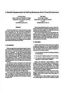
B2 -segment α = [68 : 89] (horizontal axis) as well as the induced segment family (vertical axis). The induced segmentation consists of four segments corresponding to the four occurrences of the B-part in this recording. Note that repeating segments may be played in different tempi. For example, the B2 -part is played much faster than the B1 part. Similarly, Figure 1d shows the optimal path family for the segment α = [131 : 150] (corresponding to the A3 part) and the induced segmentation (consisting of the three A-part segments). Finally, Figure 1e reveals that, for the long segment α = [131 : 196] (corresponding to A3 B3 B4 ), there exists a similar segment (corresponding to A2 B1 B2 ). The fitness value of a given segment is derived from the corresponding optimal path family and the values of the underlying SSM. Intuitively, one considers the overall score accumulated by the path family and the total length covered by the induced segmentation. After a suitable normalization, the fitness is defined as the harmonic mean of of coverage and score. For further details, we refer to [10].
−2
Time (sec)
Figure 1: Various representations for an Ormandy recording of Brahms’ Hungarian Dance No. 5. (a) Musical form A1 A2 B1 B2 CA3 B3 B4 . (b) Fitness scape plot. The remaining subfigures show the SSM with optimal path families for various segments α (horizontal axis) and induced segment families (vertical axis). (c) α = [68 : 89] (thumbnail, maximal fitness, corresponding to B2 ). (d) α = [131 : 150] (corresponding to A3 ). (e) α = [131 : 196] (corresponding to A3 B3 B4 ).
2.1 Fitness Measure Let [1 : N ] = {1, 2, . . . N } denote the (sampled) time axis of a given music recording. Then a segment is a subset α = [s : t] ⊆ [1 : N ] specified by its starting point s and its end point t. Let |α| := t−s+1 denote the length of segment α. In [10], a fitness measure has been introduced that assigns to each audio segment α a fitness value ϕ(α) ∈ R which simultaneously captures two aspects. Firstly, it indicates how well the given segment explains other related segments. Secondly, it indicates how much of the overall music recording is covered by all these related segments. In the computation of the fitness measure, an enhanced self-similarity matrix (SSM) is computed from the music recording based on chroma-based audio features. It is well known that each path of the SSM (a stripe of high score running parallel to the main diagonal) reveals the similarity of two segments (given by the two projections of the path onto the vertical axis and horizontal axis), see [13]. The main idea of [10] is to compute for each audio segment α a so-called optimal path family over α that simultaneously reveals the relations between α and all other similar segments. By projecting such optimal path family to the vertical axis, we get the corresponding induced segment family, where each element of this family defines a segment similar to α. As an example, we consider a recording of the Hungarian Dance No. 5 by Johannes Brahms, which has the musical form A1 A2 B1 B2 CA3 B3 B4 , see Figure 1a. Figure 1c shows an optimal path family (cyan stripes) for the
2.2 Scape Plot Representation We now describe how a compact fitness representation for the entire music recording can be obtained showing the fitness ϕ(α) for all possible segments α. Note that each segment α = [s : t] is specified by its center c(α) := (s+t)/2 and its length |α|. Using the center as horizontal coordinate and the length as vertical coordinate, each segment can be represented as a point in some triangular representation also referred to as scape plot. Such scape plots were original introduced by Sapp [14] to represent harmony in musical scores in a hierarchical way. In our context, we define a scape plot Φ by setting Φ(c(α), |α|) := ϕ(α) for segment α. Figure 1b shows a visualization of the fitness scape plot for our Brahms example, where the fitness is represented by a lightness grayscale ranging from white (fitness is zero) to black (fitness is high). The points corresponding to the three segments discussed above are marked within the scape plot by small circles. For example, the segment α = [68 : 89] (corresponding to B2 ) has the scape plot coordinates c(α) = 78.5 (horizontal axis) and |α| = 22 (vertical axis). Actually, this segment has the highest fitness among all possible segments and is also referred to as thumbnail [10]. The fitness scape plot represents the repetitiveness of each segment in a compact and hierarchical form. For example, in our Brahms example, the repeating segments corresponding to the A-parts and B-parts are reflected by local maxima in the scape plot. Also the repetitions of the superordinate segments corresponding to ABB are captured by the plot. However, so far, the visualization of the fitness scape plot does not reveal the relations across different segments. In other words, nothing is said about groups of pairwise similar segment corresponding to the various musical parts.
α
3. STRUCTURE SCAPE PLOT
(a) 0
Actually, the grouping information is implicitly encoded by the optimal path families underlying the fitness measure. To make these relations more explicit, we now extend the grayscale of the fitness scape plot by a color component that reflects the cross-segment relations. Based on the induced segmentations, we first introduce a distance measure that allows for comparing two arbitrary segments (Section 3.1). Then the objective is to map similar segments to similar colors and dissimilar segments to distinct colors. In the following, we proceed in several steps including a color mapping step (Section 3.2), a point sampling and interpolation step (Section 3.3), and a color combination step (Section 3.4). The overall pipeline of our procedure is also illustrated by Figure 4.
20
40
60
80
100
120
140
160
180
200
200
β (b) 0
20
40
60
α1
80
100
120
140
α2
160
180
α3
α4
160
180
200
180
200
(c) 0
20
40
60
80
100
120
140
β1
β2
(d) 0
20
40
60
80
100
120
140
160
Time (sec)
Figure 2: Illustration of the computation of the distance measures δ(α, β) used to compare two segments α (shown in (a)) and β (shown in (b)). The respective induced segment families are shown in (c) and (d), respectively. The black box indicates the union and the red box the overlap of the two segments which are used to compute distance value δ(α, β). 1
3.1 Segment Distance Measure Recall from Section 2.1 that for a given segment α there is an optimal path family along with an induced segment family, where each segment of this family is similar to α. Let A = {α1 , α2 , . . . , αK } denote the induced segment family of α, then the segments αk , k ∈ [1 : K], can be thought of as the (approximate) repetitions of α. Note that, by definition, overlaps between repetitions are not allowed, see [10]. Now, let α and β be two arbitrary segments. Intuitively, we consider these two segments to be close if they are approximately repetitions of each other (or at least if some repetitions of α and β have a substantial overlap), otherwise α and β are considered to be far apart. More precisely, let A = {α1 , . . . , αK } and B = {β1 , . . . , βL } be the respective induced segment families. Then, we define the distance δ(α, β) between α and β to be δ(α, β) := 1 −
max
k∈[1:K],ℓ∈[1:L]
|αk ∩ βℓ | , |αk ∪ βℓ |
(1)
see also Figure 2 for an illustration. In other words, the distance is obtained by subtracting the maximal overlap (relative to the union) over all repetitions of α and β from the value 1. For example, the B1 -segment and B2 -segment for the Brahms recording have a small distance (close to zero) since the induced segment families more or less coincide (consisting of the four B-part segments). In contrast the B1 -segment and the A1 -segment have a large distance (close to one) since none of their repetitions have a substantial overlap. 3.2 Color Mapping Based on the distance measure δ, we now introduce a procedure for mapping the scape plot points (segments) to color values in such a way that distance relations are preserved. To this end, we first need to specify a suitable color space. Because of its perceptual relevance, we revert to the HSL model, which is a cylindric parametrization of the RGB color space [6]. Here the angle coordinate H ∈ [0, 360] (given in degrees) refers to the hue, the coordinate S ∈ [0, 1] to the saturation, and the coordinate
L 0
0◦
120◦
H
240◦
360◦
Figure 3: Cylindric HSL (hue, saturation, lightness) color representation. The figure shows only the outside surface of the cylinder corresponding to the saturation S = 1.
L ∈ [0, 1] (with 0 being black and 1 being white) to the lightness of the color. To obtain “full” saturated colors, we fix the parameter S = 1. Figure 3 shows the color space for S = 1 spanned by the coordinates H and L. Note that the hue angle coordinates H = 0 and H = 360 encode the same color (by definition this is the color “red”). In the following, we reserve the lightness coordinate to represent the fitness value and only use the hue coordinate to represent the cross-segment relationships. The problem of mapping the scape plot points to the hue color coordinates (which topologically corresponds to the unit circle) in a distance preserving way can be seen as an instance of multidimensional scaling (MDS), see [1]. Generally, MDS refers to a family of related techniques which allow for mapping a set of points with pairwise distance values onto a low-dimensional Euclidean space (often dimension 2 or 3 for visualization purposes) such that the distances between the original points are approximated by the Euclidean distances of the mapped points. In the following, we use basic MDS techniques to map the scape plot points onto the unit circle (representing the hue color space). Let M denote the number of scape plot points to be considered in the mapping, see Figure 4b. First, we compute an M × M -distance matrix ∆ by comparing the M points in a pairwise fashion using δ. Next, we perform a principal component analysis (PCA) of ∆ and consider the two eigenvectors corresponding to the two largest eigenvalues. The columns of ∆ (which are indexed by the M scape plot points) are then projected onto the two-dimensional Euclidean space defined by these two eigenvectors, see Figure 4c. Using PCA, the variance across the mapped column vectors is maximized. Therefore, scape plot points that have a distinct distance distri-
(a)
(c)
200
(g)
(e) 200
8
Segment length (sec)
Segment length (sec)
6 150
4 2 0
100
−2 −4
50
−6
150
100
−8 0
0
50
100
150
200
−8
−6
−4
−2
0
2
4
6
8
Segment center (sec)
Segment center (sec)
(b)
(d)
(f) 200
Segment length (sec)
Segment length (sec)
200
150
100
50
0
0
50
100
150
200
50
150
9 0
100
0
50
A1
A2
B1
100
B2
150
C
A3
200
B3
B4
50
9 0
0 0
Segment center (sec)
50
100
150
200
50
100
150
200
Time (sec)
Segment center (sec)
Figure 4: Illustration of the pipeline for computing the structure scape plot for Brahms. (a) Fitness scape plot. (b) Fitness scape plot with sampled anchor points. (c) Anchor points projected onto the first two principal components. (d) Anchor points projected to the unit circle colored with the resulting hue value. (e) Hue-colored anchor points. (f) Hue-colored scape plot using interpolation techniques. (g) Structure scape plot combining fitness (lightness) and cross-segment relation (hue) information.
bution to the other points (encoded by its respective column vectors) are likely to be mapped to different regions in the 2D space, see [1] for details. Furthermore, as shown in Figure 4c, the projected points are usually distributed in a circular fashion (even though this is not guaranteed and crucially depends on the distance distributions of the original points). Finally, we normalize the projected points with respect to the Euclidean norm to obtain points on the unit circle, which yields angle parameters that are associated to hue values, see Figure 4d. Figure 4e shows the original scape plot points colored with the derived hue values. 3.3 Sampling and Interpolation Using all scape plot points in the described color mapping procedure may be problematic because of two reasons. Firstly, using a large number M of points would not only make the computation of the M × M distance matrix ∆ but also of the subsequent PCA rather expensive. Therefore, the number M of used points should be kept small. Secondly, using all scape plot points may over-represent segments of short lengths that are located in the lower part of the triangular scape plot. As a result, the distance relations of the short segments may dominate the selection of the eigenvectors obtained in the PCA step. Therefore, we only choose a suitable subset of scape plot points, also referred to as anchor points, and then transfer the obtained hue color information to the other points using interpolation techniques. Note that scape plot points of higher fitness are structurally more relevant than scape plot points of lower fitness. Therefore, in the anchor point selection step, we sample the scape plot by taking the fitness into account. To this end, we use a greedy procedure that consists of two steps. Firstly, we select the scape plot point of maximal fitness as an anchor point. Secondly, around this anchor
point, we specify a neighborhood of size ρ > 0 and set the fitness values of all points in this neighborhood to zero excluding them for the subsequent procedure. The role of the neighborhood is to avoid a sampling that is locally too dense. This procedure is repeated until either all of the remaining scape plot points have a fitness of zero, or until a specified maximal number of points M0 is reached, see also Figure 4b. Sometimes the fitness values of short segments are rather “noisy.” This may also have musical reasons since such segments often correspond to highly repetitive fragments like a short riff or a single chord of dominant harmony. Therefore, it is often beneficial to exclude such short segments in the anchor point selection by only considering scape plot points whose length coordinate lies above a certain lower bound λ > 0. The influence of the parameters M0 , ρ, and λ on the resulting number of anchor points M is discussed in Section 4. The color mapping as described in Section 3.2 is now applied only to the anchor points. In the next step, the color information is transferred to arbitrary scape plot points by simply interpolating color values of the nearest neighborhood anchor points. However, since the hue values live on a unit circle (rather than in the two-dimensional Euclidean space), one needs to use spherical interpolation instead of linear interpolation. Figure 4f shows the interpolation result obtained from the anchor points of Figure 4e. 3.4 Color Combination So far, we have derived two scape plot visualizations: one indicating the repetitive properties (fitness value represented by lightness, see Figure 4a) and the other indicating the cross-segment relations (represented by hue colors, see Figure 4f). We now combine this information within a single scape plot representation, which we also refer to as
(a)
(b)
250
Chopin, where we manually generated some structure annotations for each piece. Note that these annotations are not needed to generate the structure scape plots, but are only used to compare our visualizations with some sort of ground truth. As mentioned in the introduction, the purpose of the scape plot visualizations is to yield a compact and intuitive representation without the necessity of explicitly extracting the structure.
250 200 200
150 150
100
100
50
13 0
50 19 0
50
100
150
200
0
250
0
A1B1A2B2A3 C D1 D2 A4B3A5 0
(c)
50
100
150
200
250
100
50
100
150
200
I V1 B1 V2 V3 B2 V4 0
(d)
50
100
150
200
250
O 250
150
90 80 70
100 60 50 40
50
30 20 10 4 0
10 0
20
A1 0
40
60
B1 B2 20
40
80
100
A2 60
Time (sec)
80
0
0
50
100
150
I V1 V2 B1 V3 V4 B2 V5 O 100
0
50
100
150
Time (sec)
Figure 5: Structure scape plots and structure annotations for recordings of various pieces. (a) Chopin Mazurka Op. 17 No. 3. (b) Beatles song “While My Guitar Gently Weeps.” (c) Chopin Mazurka Op. 33 No. 3. (d) Beatles song “You Can’t Do That.”
structure scape plot. To this end, we first linearly map the fitness values onto the lightness parameter space [0, 1] of the HSL model such that L = 1 (white) corresponds to the fitness value 0 and L = 0 (black) to the maximal fitness value occurring in the fitness scape plot. Furthermore, by rotating the hue parameter space (unit circle) we normalize the color assignment such that the thumbnail (fitnessmaximizing scape plot point) is mapped to the color “red” (angle H = 0). Finally, for each scape plot point we use the saturation S = 1, the computed lightness L, and the normalized hue angle H to obtain a single color value. Figure 4g shows the final result of the structure scape plot for our Brahms example. Note that the four B-part segments (repetitions of the B2 -thumbnail) are represented by red, the three A-part segments by blue, and the superordinate two ABB-part segments by green. Furthermore, the visualization reveals some substructures of the A-parts, each actually consisting of two (approximate) repetitions. Finally, note that smaller segments within the C-part are assigned to the color violet. Since the C-part contains many fragments sharing the same harmony, our procedure has captured some repetitiveness also in this middle part. 4. EXAMPLES AND DISCUSSION In this section, we indicate the potential and some limitations of our visualization procedure by discussing representative examples. In our experiments, we used audio recordings considering popular music as well as classical music. On the one hand, we employed the dataset consisting of recordings of the 12 studio albums by “The Beatles” using the structure annotations as described by [9]. On the other hand, we used the complete Rubinstein (1966) recordings of the 49 Mazurkas composed by Fr´ed´eric
As for the parameter settings, we choose M0 , ρ, and λ in a relative fashion depending on the duration of the respective music recording. In particular, we determined the upper bound M0 and the neighborhood parameter ρ to result in a number M of anchor points ranging between 200 and 250 for each recording. Furthermore, the lower bound λ was set to correspond to 5-7 % of the recording’s total duration. Figure 5 shows structure scape plots for some representative music recordings. For example, Figure 5a shows the scape plot for a Rubinstein performance of Chopin’s Mazurka Op. 17 No. 3. The five A-part segments, which also comprise the thumbnail, are represented by red. Furthermore, the three B-part segments are indicated by a lighter orange color, and the superordinate ABA-part segments are represented by green. Also substructures of the A-part segments are visible: indeed each A-part consists of two similar subparts. Interestingly, the segments corresponding to the C- and the two D-parts are all represented by pink. Actually this is musically meaningful, since each of the two repeating D-parts is only a slight extension of the C-part. Figure 5b visualizes the structure scape plot for the Beatles song “While My Guitar Gently Weeps.” Also in this example, the structure scape plot nicely reflects the overall musical form. Each of the four verse segments (V part) consists of two (approximately) repeating subparts, say V = W W . Actually, the intro also corresponds to such a subpart (I = W ) and the outro corresponds to three of these subparts (O = W W W ), which also explains the red coloring of these segments. Furthermore, the color blue corresponds to W W W -segments and the color green to V BV -segments. The structure scape plot of a recording of the Mazurka Op. 33 No. 3 is shown in Figure 5c, which indicates a number of substructures not reflected in the structure annotation (see both A parts). Finally, Figure 5d correctly reproduces the overall structure of the Beatles song “You Can’t Do That.” Only the V4 -segment has not been captured well. Actually, V4 corresponds to an instrumental section with some vocal interjections, which make the V4 segment spectrally quite different to the other four V -part segments. Next, we discuss some limitations and problems that may occur in our visualization approach. As an illustrating example, we consider the Beatles song “Hello Goodbye.” Figure 6b shows the structure scape plot using our standard parameter setting as described above. The red color corresponds to the four V R-part segments, which also comprise the thumbail. However, the individual V -part and R-part segments are all represented by green and are not distin-
(a)
(b)
6
200 180 160
3
140 120 0
100 80 60
−3
40 20 14
−6 −6
−3
0
3
0
6
0
50
100
150
V1 R1 V2 R2 V3 R3 V4R4 F 0
(c)
(d)
6
50
100
200
S
150
200
200 180 160
3
better represent more complex structures. So far, we have only given a qualitative evaluation to demonstrate the potential of our techniques. In this context, user studies may be necessary to better understand the actual user needs and the applicability of our concepts. Besides introducing a novel segment distance function as well as a grouping and coloring procedure, the main contribution of this paper was to introduce the concept of a structure scape plot for visualizing repetitive structures of music recordings. We hope that our visualization is not only aesthetically appealing, but also may allow a user to explore and browse musical structures in novel ways.
140 120
0
Acknowledgments: This work has been supported by the Cluster of Excellence on Multimodal Computing and Interaction at Saarland University and the German Research Foundation (DFG MU 2686/5-1).
100 80 60
−3
40
−6 −6
−3
0
3
6
20 10 0
6. REFERENCES 0
50
100
150
V1 R1 V2 R2 V3 R3 V4R4 F 0
50
100
150
200
S 200
Time (sec)
Figure 6: Anchor points projected onto the first two principal components (left) and resulting structure scape plot (right) for the Beatles song “Hello Goodbye.” (a)/(b) Using λ = 14 seconds. (c)/(d) Using λ = 10 seconds.
guishable. The reason for this is that the lower bound for the anchor points was set to λ = 14 seconds, which is too high to capture the finer structures. By decreasing this parameter to λ = 10 seconds, V -part and R-part segments are separated, see Figure 6d. As this example shows, the choice of the parameter λ may have a significant impact on the final visualization. The Beatles example also indicates a second problem that may arise in our color mapping procedure. Usually, the anchor points projected to the two principal components are homogeneously distributed along the unit circle as in our Brahms example, see Figure 4c. Therefore, projecting these points to the unit circle (to yield the desired hue values) does not destroy too much of the neighborhood relations. However, in the Beatles example, the projected anchor points are rather scattered in the two-dimensional Euclidean space with some outliers as indicated by the boxed and circled points shown in Figure 6a. Therefore, projecting these points onto the unit circle may result in the same hue value for anchor points that are actually far apart. This explains, why the substructures within the S-part are mapped to the same color as substructures of the V R-part, see Figure 6b. 5. FUTURE WORK These problems indicate some future research directions. Possible improvements of the color mapping step may be achieved by applying more involved generalized multidimensional scaling techniques which directly map the anchor points to a smooth manifold (in our case the unit circle). Also, the one-dimensional hue color space may not suffice to suitable capture more intricate cross-segment relations. Here, a more flexible usage of the color space or an extension to 3D scape plot representations may help to
[1] Ingwer Borg and Patrick J. F. Groenen. Modern Multidimensional Scaling Theory and Applications. Springer, 2005. [2] Matthew Cooper and Jonathan Foote. Summarizing popular music via structural similarity analysis. In Proc. IEEE Workshop on Applications of Signal Processing to Audio and Acoustics (WASPAA), pages 127–130, New Paltz, NY, USA, 2003. [3] Roger B. Dannenberg and Masataka Goto. Music structure analysis from acoustic signals. In David Havelock, Sonoko Kuwano, and Michael Vorl¨ander, editors, Handbook of Signal Processing in Acoustics, volume 1, pages 305–331. Springer, New York, NY, USA, 2008. [4] Jonathan Foote. Visualizing music and audio using self-similarity. In Proc. ACM International Conference on Multimedia, pages 77–80, Orlando, FL, USA, 1999. [5] Masataka Goto. A chorus section detection method for musical audio signals and its application to a music listening station. IEEE Trans. Audio, Speech and Language Processing, 14(5):1783–1794, 2006. [6] Allan Hanbury. Constructing cylindrical coordinate colour spaces. Pattern Recognition Letters, 29:494–500, 2008. [7] Mark Levy, Mark Sandler, and Michael A. Casey. Extraction of high-level musical structure from audio data and its application to thumbnail generation. In Proc. IEEE International Conference on Acoustics, Speech, and Signal Processing (ICASSP), pages 13–16, Toulouse, France, 2006. [8] Namunu C. Maddage. Automatic structure detection for popular music. IEEE Multimedia, 13(1):65–77, 2006. [9] Matthias Mauch, Chris Cannam, Matthew E.P. Davies, Simon Dixon, Christopher Harte, Sefki Kolozali, Dan Tidhar, and Mark Sandler. OMRAS2 metadata project 2009. In Late Breaking Demo, International Conference on Music Information Retrieval (ISMIR), Kobe, Japan, 2009. [10] Meinard M¨uller, Peter Grosche, and Nanzhu Jiang. A segment-based fitness measure for capturing repetitive structures of music recordings. In Proc. 12th International Conference on Music Information Retrieval (ISMIR), pages 615–620, Miami, FL, USA, 2011. [11] Meinard M¨uller and Frank Kurth. Towards structural analysis of audio recordings in the presence of musical variations. EURASIP Journal on Advances in Signal Processing, 2007(1), 2007. [12] Jouni Paulus and Anssi P. Klapuri. Music structure analysis using a probabilistic fitness measure and a greedy search algorithm. IEEE Trans. Audio, Speech, and Language Processing, 17(6):1159–1170, 2009. [13] Jouni Paulus, Meinard M¨uller, and Anssi P. Klapuri. Audio-based music structure analysis. In Proc. 11th International Conference on Music Information Retrieval (ISMIR), pages 625–636, Utrecht, The Netherlands, 2010. [14] Craig Stuart Sapp. Harmonic visualizations of tonal music. In Proc. International Computer Music Conference (ICMC), pages 423–430, 2001. [15] Ho-Hsiang Wu and Juan P. Bello. Audio-based music visualization for music structure analysis. In Proceedings of Sound and Music Computing Conference (SMC), Barcelona, Spain, 2010.