A Self-Learning Sensor Fault Detection Framework for Industry ...

Hindawi Publishing Corporation Mathematical Problems in Engineering Volume 2013, Article ID 712028, 8 pages http://dx.doi.org/10.1155/2013/712028

Research Article A Self-Learning Sensor Fault Detection Framework for Industry Monitoring IoT Yu Liu,1 Yang Yang,2 Xiaopeng Lv,3 and Lifeng Wang4 1

State Key Laboratory of Software Development Environment, Beihang University, Beijing 100191, China Information Center of Guangdong Power Grid Corporation, China Southern Power Grid, Guangzhou 510620, China 3 Beijing Guotie Huachen Communication & Infomation Technology Co., Ltd., Beijing 10070, China 4 Beijing Electronic Science and Technology Institute, Beijing 100070, China 2

Correspondence should be addressed to Yu Liu; [email protected] Received 8 June 2013; Accepted 3 August 2013 Academic Editor: Zhongmei Zhou Copyright © 2013 Yu Liu et al. This is an open access article distributed under the Creative Commons Attribution License, which permits unrestricted use, distribution, and reproduction in any medium, provided the original work is properly cited. Many applications based on Internet of Things (IoT) technology have recently founded in industry monitoring area. Thousands of sensors with different types work together in an industry monitoring system. Sensors at different locations can generate streaming data, which can be analyzed in the data center. In this paper, we propose a framework for online sensor fault detection. We motivate our technique in the context of the problem of the data value fault detection and event detection. We use the Statistics Sliding Windows (SSW) to contain the recent sensor data and regress each window by Gaussian distribution. The regression result can be used to detect the data value fault. Devices on a production line may work in different workloads and the associate sensors will have different status. We divide the sensors into several status groups according to different part of production flow chat. In this way, the status of a sensor is associated with others in the same group. We fit the values in the Status Transform Window (STW) to get the slope and generate a group trend vector. By comparing the current trend vector with history ones, we can detect a rational or irrational event. In order to determine parameters for each status group we build a self-learning worker thread in our framework which can edit the corresponding parameter according to the user feedback. Group-based fault detection (GbFD) algorithm is proposed in this paper. We test the framework with a simulation dataset extracted from real data of an oil field. Test result shows that GbFD detects 95% sensor fault successfully.

1. Introduction Internet of Things (IoT) has been paid more and more attention by the government, academe, and industry all over the world because of its great prospect [1–3]. In the IoT application field, intelligent industry is an important branch. A wired or wireless sensor network is the basic facility of the industry monitoring IoT. These networks comprising of thousands of inexpensive sensors can report their values to the data center. The aim of the monitoring system is to guarantee the process of production. Fault detection is an important process for industry monitoring IoT, but it is a difficult and complex task because there are many factors that influence data and could cause faults. And faults are application and sensor type dependent [4–6]. Sensors in an industry monitoring IoT have three features:

(1) Big: thousands of sensors on different devices are working together, (2) Multitypes: many physical quantities are needed to determine the production status, (3) Uncertainty: different workload is needed according to the production plan and some devices need shut down for examination. So the values of correlative sensors will change between different levels. From the data-centric view, we focus on the Outliers, Stuck-at faults and Spikes [7]. From the application and system view, we focus on the rational and irrational trend detections. A rational trend means the sensor value transforms from one level to another smoothly and it is caused by a rational reason, such as shut down a device. An irrational trend means value changed when something is wrong with a device. The typical two mistakes of the monitoring system are taking a rational trend for an Outlier, or ignoring an irrational trend while values are still in range.

2

Mathematical Problems in Engineering 100 Sensor value (KPa for P and ∘ C for T)

Vc

Value

Vc−m

Wk

···

W3

W2

W1 Wr Wc

Time

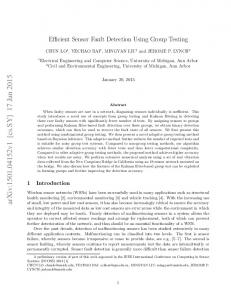
Figure 1: Estimation of the data distribution in the Statistics Sliding Windows (SSW) for one time instance. L L-1-1

P-8 V-1 E-1

V-5 P P-0-1

T T-0-1

L L-2-1

V-2 E-2

V-3 E-3

L L-3-1

P-1 P P-1-1

T T-1-1 P-2

P P-2-1

T T-2-1 P-3

P P-3-1

T T-3-1

Figure 2: Typical flowchat of a gas processing plant.

In this paper, we propose a self-learning sensor fault detection framework for industry monitoring IoT. The data model design is described in Section 3. In Section 4, the framework and the core algorithm are discussed. A simulation experiment base on real data is shown in Section 5.

2. Related Work Many researchers pay their attention to building a smart monitoring system. Bressan et al. [8] created a solid routing infrastructure through RPL. Castellani et al. [9] concentrate on the actual implementation of the communication technology and presented a lightweight implementation of an EXI library. Yuan et al. [10] present a parallel distributed structural health monitoring technology based on the wireless sensor network. An IoT communication framework for distributed worldwide health care applications is maintained in [11]. All these works are focused on the basic frameworks, protocols, and communication technologies of monitoring systems but discussed less on sensors management. For modeling sensor network data, Guestrin et al. [12] propose a framework, for the nodes in the network to collaborate in order to fit a global function to each of their local measurements. This is a parametric approximation technique

90 80 70 60 50 40

Status transform window

30 20 10 0

0

10

20

30 Time (s)

40

50

60

Pressure P1 Pressure P2 Temperature T1

Figure 3: Status transformation process for two time instances.

and has more parameters then our approach. References [13, 14] study the problem of computing order statistics in a sensor network. There has also been work on predicting and caching the values generated by the sensors [15, 16], which can result in significant communication savings. But all these approaches are not fit our setting. A similar approach for sensor fault detection in streaming data is described by Yamanishi et al. [17]. In contrast to our work, their method does not operate on sliding windows but rather on the entire history of the data values. Chan et al. [18] extend the study of algorithms for monitoring distributed data streams from whole data streams to a time-based sliding window, but their focus is on presenting a communicationefficient algorithm. Ding et al. [19] combined trajectories of all nodes and the paramealgorithm which requires low computational overhead. The proposed algorithm compared its sensor reading with the median value of its neighbors’ readings. Gao et al. [20] approach WSN fault detection problems using spatial correlation with the assumption of similar reading within cross range of neighbor nodes. Krishnamachari and Iyengar [21] tried to solve the faulty node detection problem by using localized event region and they assume that the system knows the location of sensor. In an industry monitoring sensor network, finding out a neighbor automatically is very hard. In our approach, we separate sensors into groups according to the production flow charts.

3. Data Model Design This section focuses on the sensor data model design. We model sensors from the view of value for Outliers, Stuck-at faults, and Spikes detection and from the application view for event detection. The events we are interested in are rational trend and irrational trend.

Mathematical Problems in Engineering

Input sensor value (ID, value)

3

Self-learning sensor fault detection Detection thread Thread status queue Parameter filter Working threads pool

Self-learning thread

Iterate

Task timer

Outlier

Stuck

Status trend

Spikes

Feature selection Sensor fault warning Trend vector

NB classification

Incremental clustering Application DB

Parameter feedback

Output interface DB operation Control ﬂow I/O interface

Figure 4: A self-learning sensor fault detection framework.

3.1. Sensor Value. For detection the Outliers, Stuck-at faults, and Spikes, we propose a statistics method. Figure 1 shows the mechanism of Statistics Sliding Windows (SSW). For sensor 𝑠, the current value V𝑐 and the previous 𝑚 values form the current windows 𝑊𝑐 = {V𝑐−𝑚 , V𝑐−𝑚+1 , V𝑐−𝑚+2 , . . . , V𝑐 }. In the recent history, we can define 𝑘 windows with the same length and get the set 𝐻V = {𝑊1 , 𝑊2 , 𝑊3 , . . . , 𝑊𝑘 }. We estimate the values in each sliding window by Gaussian distribution, 𝑊𝑖 → 𝑁(𝜇𝑖 , 𝜎𝑖2 ) (Formula (1)). If 𝜎𝑐2 = 0, a Stuck-at fault is detected. And when 𝜎𝑐2 is big enough, a Spikes fault may happened: 𝑊𝑖 󳨀→ 𝑁 (𝜇, 𝜎2 ) , 𝜇=

∑𝑚 𝑘=1 V𝑘 , 𝑚

𝜎2 =

2

∑𝑚 𝑘=1 (V𝑘 − 𝜇) . 𝑚

(1)

There is a buffer named 𝑊𝑟 in front of the current window 𝑊𝑐 . With the new samples coming into 𝑊𝑐 , the obsolete samples deserted by 𝑊𝑐 will become a member of 𝑊𝑟 . When the size of 𝑊𝑟 reach 𝑚, the oldest window in 𝐻V will be discarded and the current 𝑊𝑟 will join 𝐻V as 𝑊1 . With SSW, large numbers of historical sensor values are regressed to 𝑘 pairs of Gaussian characteristics. In a real application, we need not hold all the recent values in the memory. 3.2. Status Group. In the industry monitoring IoT, the status of a production line may be uncertain. With the different manufacturing techniques and different workloads, some devices in the production line may be shut down. In this case, the whole production line is still working, but values of sensors monitoring the shutdown devices will run out of

range (Outliers). At the same time, related devices may also change with the shutting down operation. In an industry monitoring IoT, the rational status transformation of sensors should be recognized and ignored. Figure 2 shows a typical flow chat of a gas-processing plant. P-1, P-2, and P-3 are three parallel subpipelines which are controlled by V-1, V-2, and V-3, respectively. Each subpipeline can be shut down independently and this operation will affect the value of P-0-1, a pressure sensor on the main input pipeline. In our approach, we deposit the sensors in the goal-processing plant into several status groups. Although the application background is important to the disposition method, we can follow some common rules as follows: 𝐺 = {𝑆1 , 𝑆2 , . . . , 𝑆𝑛 } ,

𝑆𝑖 ∈ VALVE𝑃 , 𝑛 ≤ 10.

(2)

(1) Sensors on the opposite side of a valve are not in the same group. A valve is a typical controller in the industrial IoT. All the devices on the backward position can be shut down by the proper valve. The sensors on the different side may be in different status. (2) If there are too many sensors which are controlled by one slave, they should be divided into different groups. In our approach, we will not put more than 10 sensors into one status group because the probable status space will expand acutely with the increasing sensor numbers. In this case, sensors can be grouped by their relative position with the most complex device, because the complex device may lead to status change most possibly.

4

Mathematical Problems in Engineering (1) let 𝑊𝑚 be the statistics sliding windows size; (2) let 𝜀𝑠 be the outlier detection threshold for sensor S and let P be the global list to keep all of the 𝜀𝑠 ; (3) let U and V be the global arrays to keep the last 10 gaussian distribution characteristics for each sensor; (4) let 𝑊𝑛 be the status transform windows size and 𝜃𝑖 /4 be the trend vector merging threshold for group 𝐺𝑖 , all the rational trend vectors of 𝐺𝑖 are stored in 𝑅𝑖 ; (5) procedure GFD () (6) init P, loading 𝜀 from Appilcation DB; (7) init U and V, loading the last 10 distribution characteristics from Application DB; (8) create C DetectionThread threads, 𝐶 = 𝑁𝑢𝑚𝑐𝑝𝑢 ∗ 2; (9) start SelfLearningThread(); (10) do (11) get a value set V𝑖 for sensors in a group 𝐺𝑖 ; (12) find a idle DetectionThread; (13) DetectionThread(V𝑖 ); (14) while not end; (15) return; (16) procedure DetectionThread(V𝑖 ) (17) if (IsStuck(V𝑖 ) or IsSpikes(V𝑖 )) (18) return; (19) if (IsOutlier(V𝑖 ) and not IsRatStatChange(V𝑖 )) (20) return; (21) IsRatStatChange(V𝑖 ); (22) return; (23) procedure IsStuck(V𝑖 ) (24) get 𝜎𝑖𝑗 2 for sensor j by 𝑇𝑐 ; (25) if (𝜎𝑖𝑗 2 = 0) (26) mark 𝑠𝑖𝑗 as a Stuck; (27) return; (28) procedure IsSpikes(V𝑖 ) (29) get 𝜇𝑖𝑗 and 𝜎𝑖𝑗 2 for sensor j by 𝑇𝑐 ; (30) if (𝜇𝑖𝑗 /mean(𝑈(𝜇𝑖 )) < 𝜉 and 𝜎𝑖𝑗 2 /mean(𝑉(𝜎𝑖 2 )) > 𝜏) (31) mark 𝑠𝑖𝑗 as a Spikes; (32) return; (33) procedure IsOutlier(V𝑖 ) (34) use U and V to caculate 𝜃𝑖𝑗 ; (35) if (𝜃𝑖𝑗 > 𝜀𝑖𝑗 ) mark 𝑠𝑖𝑗 as an Outlier; (36) return; (37) procedure IsRatStatChange(V𝑖 ) (38) use the last 𝑛 values of 𝑠𝑖 to fit the trend vector 𝑆𝑖 ; (39) for each rational trend 𝑟𝑖 in 𝑅𝑖 (40) if (cosine(𝑟𝑖 , 𝑆𝑖 ) < 𝜃𝑖 /4) (41) mark 𝑆𝑖 as a rational status change; 𝑆𝑖𝑗 = mean(𝑆𝑖𝑗 , 𝑟𝑖𝑗 ); (42) mark the max unstable sensor 𝑠𝑖𝑗 as a sensor falut; (43) return; (44) procudure SelfLearningThread() (45) while (true) do: (46) load the user feedback; (47) for each miss alart (48) if missed Outlier then 𝜀𝑖𝑗 = 𝜀𝑖𝑗 ÷ 𝜆; (49) if missed irrational status change then 𝜃𝑖 = 𝜃𝑖 × 𝜆; (50) IncClustering(𝑆𝑖 , null); (51) for each false alart (52) if false Outlier then 𝜀𝑖𝑗 = 𝜀𝑖𝑗 × 𝜆; (53) if false irrational status change then 𝜃𝑖 = 𝜃𝑖 ÷ 𝜆; (54) IncClustering(𝑆𝑖 , 𝑟𝑖𝑗 ); (55) sleep(𝑇); continues; Algorithm 1: Continued.


5

(56) return; (57) procedure IncClustering(𝑆𝑖 ,𝑟𝑖𝑗 ) (58) if 𝑟𝑖𝑗 is not null then for each 𝑆𝑖𝑗 in 𝑆𝑖 ; (59) if there is cosine(𝑟𝑖 , 𝑆𝑖 ) < 𝜃𝑖 then 𝑆𝑖𝑗 = mean(𝑆𝑖𝑗 , 𝑟𝑖𝑗 ); (60) else add 𝑟𝑖𝑗 into 𝑆𝑖 ; (61) for each two 𝑆𝑖𝑗 , 𝑆𝑖𝑘 in 𝑆𝑖 ; (62) if (cosine(𝑆𝑖𝑗 , 𝑆𝑖𝑘 ) < 𝜃𝑖 ) (63) 𝑆𝑖𝑗 = mean(𝑆𝑖𝑗 , 𝑆𝑖𝑘 ); remove 𝑆𝑖𝑘 ; (64) return; Algorithm 1: A group-based fault detection Algorithm.

(3) The production line is normally divided into many units according to the geographical position. We can ignore the relationship between sensors in different sections. For the 11 sensors shown in Figure 2, we divide them into four groups which are 𝐺0 = {𝑃0−1 , 𝑇0−1 }, 𝐺1 = {𝑃1−1 , 𝐿 1−1 , 𝑇1−1 }, 𝐺2 = {𝑃2−1 , 𝐿 2−1 , 𝑇2−1 }, and 𝐺3 = {𝑃3−1 , 𝐿 3−1 , 𝑇3−1 }. 𝐺0 represents the status of the main input pipeline. 𝐺1 , 𝐺2 , and 𝐺3 are status groups which are derived from the three parallel subpipelines respectively. 3.3. Status Model. For a status group 𝐺 = {𝑆1 , 𝑆2 , . . . , 𝑆𝑛 }, all the sensors in 𝐺 may have different trends when the production status changed. Figure 3 shows a status transformation process. 𝑃1 , 𝑃2 , and 𝑇1 are stable in the first 30 and the last 20 seconds. The interval from 30 s to 40 s is called the Status Transform Window (STW). 𝑃1 and 𝑃2 increase to a new level while 𝑇1 keep the same trend. And the slopes of 𝑃1 and 𝑃2 are different. We use the trend vector which contains all the slopes of one sensors’s group to represent the status transformation, that is, 𝑆 = {𝑘1 , 𝑘2 , . . . , 𝑘𝑛 }. The trend of a sensor can be found by fitting its values by a specific size of STW. Here, we use the least-square method [22] (Formula (3)) to fit the values and record the rational trend vector by the sensor index. We use the key idea of incremental clustering algorithm [23] to handle the trend vectors, get the cosine angle between the current trend and existing vectors, respectively. If the angle is big enough then mark it a new trend. Otherwise, a repeated trend is found and we only need to merge it with the closest vector. In Section 4, the specific clustering method will be given for details: ̂ = 𝛼 + 𝛽𝑋, ̂ 𝑌 𝛼=

∑𝑌 𝛽∑𝑋 − , 𝑛 𝑛

𝛽=

𝑛 ∑ 𝑋𝑌 − ∑ 𝑋 ∑ 𝑌 𝑛 ∑ 𝑋2

− (∑ 𝑋)

2

.

(3)

4. Design of Architecture In this section we propose the architecture for sensor fault detection in industry monitoring at first. Then, how to realize our algorithm is discussed.

Table 1: Simulation data description. Feature Sampling rate Sensor count Total samples Status groups Outliers Stuck-at & Spikes RT missed IRT missed

Value 60 s 5800 751.68 million 1340 437 163 961 35

4.1. A Self-Learning Framework. The self-learning sensor fault detection architecture is shown in Figure 4. There are four modules in our approach. (1) Application DB: all the parameters are stored in the Application DB, including the threshold 𝜀𝑠 for sensor 𝑠 and the history statistics result 𝜇𝑖 , 𝜎𝑖2 . The grouping information is also serialized in this database. This DB is the interface for high layer application which can get the sensor fault prediction and input the user feedback. (2) Detection Thread: it is a background service and contains the main detecting process. Since our approach is an online detection, a series of detection thread will be created and maintained by the working thread pool and a related status queue. When new data is coming, the working thread dispatcher a wakes up a pending thread to handle it. (3) Self-Learning Thread: the self-learning thread uses the OS timer as a driver. The user feedback about the detection result will be rechecked by this thread to revise the trend vectors. 4.2. The GbFD Algorithm. Dividing the sensors into status group is the key idea in our approach. For group-based sensor fault detection, we propose the (group-based fault detection) GbFD algorithm. The GbFD Algorithm 1 starts by initializing the global parameters (line 6-7); then it instantiates the two core processes SelfLearningThread and DetectionThread. The input

Mathematical Problems in Engineering 1

1

0.9

0.9

0.8

0.8

0.7

0.7

0.6

0.6

Recall

Precision

6

0.5

0.5

0.4

0.4

0.3

0.3

0.2

0.2

0.1

0.1

0

Set1

Set2

Set3

0

Set4 RT IRT

Otlr S&S

Set1

0.9

0.9

0.8

0.8

0.7

0.7

0.6

0.6

Recall

Precision

1

0.5

0.4

0.3

0.3

0.2

0.2

0.1

0.1 Set3

0

Set4 RT IRT

Otlr S&S

Set1

1 0.9

0.8

0.8

0.7

0.7

0.6

0.6 Recall

Precision

1

0.5 0.4 0.2

0.2

0.1

0.1

Otlr S&S (e) 𝑊𝑚 = 90, 𝑊𝑛 = 25

RT IRT

0.4 0.3

Set3

Set4

0.5

0.3

Set2

Set3

(d) 𝑊𝑚 = 60, 𝑊𝑛 = 20

0.9

Set1

Set2

Otlr S&S

(c) 𝑊𝑚 = 60, 𝑊𝑛 = 20

0

RT IRT

0.5

0.4

Set2

Set4

(b) 𝑊𝑚 = 30, 𝑊𝑛 = 15

1

Set1

Set3

Otlr S&S

(a) 𝑊𝑚 = 30, 𝑊𝑛 = 15

0

Set2

Set4 RT IRT

0

Set1

Set2

Set3

Otlr S&S

Set4 RT IRT

(f) 𝑊𝑚 = 90, 𝑊𝑛 = 25

Figure 5: Four-folder cross-validation for precision (a, c, e) and recall (b, d, f) with different 𝑊𝑚 and 𝑊𝑛 .

Mathematical Problems in Engineering of GbFD is defined as a set that contains one time samples for a status group. In the DetectionTread, we first check the Stuck-at faults and Spikes by calling the IsStuck and IsSpikes methods. And IsRatStaChange is called two times (line 19–21) to detect the sensor status transformation. When an Outlier was detected, GbFD should give the conclusion whether it is a rational operation such as shut down the device, and if no Outlier happened, we also need to check the abnormal status transformation. The first calling of IsRatStaChange is controlled by the IsOutlier method with an AND logic; no more algorithm complexity is increased by the twice calling. The SelfLearningThread works as a background service. Its responsibility is learning the user feedback to find out the missing detection and the false detection and adjusting the relational parameters. For a new rational trend vector, we will add it to the proper group rational trend history by the IncClustering method, which can recluster the grouped trend vectors according to the specified angle threshold. The time complexity of the GbFD algorithm is dominated by IsOutlier and IsRatStuChange methods. For a sensor in group 𝐺, the detection computation takes 𝑂((𝑊𝑛 + 𝑑) × 𝑊𝑚 ), 𝑊𝑛 is the STW size, 𝑑 is the length of 𝐺, and 𝑊𝑚 is the SSW size. In a real application, the two windows sizes are steerable and 𝑑 is less than 20 for the most part. Moreover, a proper thread dispatch mechanism will guarantee GbFD to handle the real-time detection task. And, the self-learning process is more complex due to many iterative operations, but it is a background service and does not require real-time performance.

5. Experimental Evaluation We built an application to evaluate our framework. This application was implemented in JAVA, about 2400 lines code and used Oracle as the Application DB. 5.1. Data Preparation. We use real data from an oil field in China. This oil field has 20 oil/gas treatment plants and all of the production equipments are monitored by sensors which can be mainly classified as temperature sensor, pressure sensor, and liquid level sensor. The sampling rate of the production IoT is 60 seconds. We obtained the sample data of 10,000 sensors between January 1st 8 PM to October 31th 8 AM, 2012. Since the production lines are relatively stable, we filtered the original data by two steps. Firstly, some production units that never make a mistake were eliminated. Secondly, for a plant, we discard some data in its stable period. Table 1 shows features of our simulation dataset. We choose more than 751 million samples from 5800 sensors. According to the corresponding flow charts, we separate the sensors into 1340 groups. Each group has 4.33 sensors in average, and the maximum group contains 8 sensors. We analyze the user feedback history and find out four typical errors. Outlier means that a value runs out of range and it is caused by the sensor failure. We put Stuck-at faults and Spikes together. The Rational Trend (RT) missed fault means that sensors submit an exceptional value after a rational user

7 operation, such as shuting down a device for examination. And the Irrational Trend (IRT) missed fault means that something wrong happened with the production line and the sensor values changed with it but still suitable with the threshold condition. 5.2. Experiment. We split the simulation data into four datasets according to the time sequence. Each time we use optional three data sets to train the GbFD algorithm and the remainder is used as the testing data. We use three pairs SSW size and STW size, which are (30, 15), (60, 20), and (90, 25), to run the four-folder crossvalidation test. The result is shown in Figure 5. When 𝑊𝑚 = 30 and 𝑊𝑛 = 15, each cross get a precision of about 80%. This result is not good enough. A satisfactory result is generated in the next test; 𝑊𝑚 = 60 and 𝑊𝑛 = 20 get a mean 95% accuracy. But with the increase of two windows size, the accuracy of GbFD will go to an opposite direction. This phenomenon indicates that the sizes of SSW and STW are strong correlating with our algorithm. Choosing the proper windows size can increase the detection sensitivity and the windows size (60, 20) is suitable with our simulation data.

6. Conclusions We present a self-learning sensor fault detection framework in this paper. We propose a model which can represent the sensor value, sensor relationship, and sensor status transformation. GbFD algorithm is proposed to detect the sensor fault. And we use real data from an oil field for validation. Experimental results show that our system can detect 95% of data fault in the simulation data which contains 751.68 million samples from 5800 sensors. We will continue validate our approach on other dataset to find out the proper statistical sliding window size and status transform windows size in different application contexts. Our goal is to build a sensor health management system for industry IoT that includes not only sensor fault detection, but also sensor lifecycle prediction and sensor inspection management.

Acknowledgments The authors would like to thank Jun Ma for helping them to dispose the simulation data. This research is supported by the National Natural Science Funds of China (61202238), the State Key Laboratory of Software Development Environment Funds (SKLSDE-2011ZX-08), and the Fundamental Research Funds for the Central Universities (2012RC0209).

References [1] Y. Liu and G. Zhou, “Key technologies and applications of internet of things,” in Proceedings of the 5th International Conference on Intelligent Computation Technology and Automation (ICICTA ’12), pp. 197–200, Zhangjiajie, China, January 2012. [2] W. Baoyun, “Review on Internet of Things,” Journal of Electronic Measurement and Instrument, vol. 23, no. 12, pp. 1–7, 2009.

8 [3] S. Haller, S. Karnouskos, and C. Schroth, “The internet of things in an enterprise context,” in Future Internet, vol. 5468 of Lecture Notes in Computer Science, pp. 14–28, Springer, Berlin, Germany, 2009. [4] I. F. Akyildiz, W. Su, Y. Sankarasubramaniam, and E. Cayirci, “A survey on sensor networks,” IEEE Communications Magazine, vol. 40, no. 8, pp. 102–105, 2002. [5] L. Paradis and Q. Han, “A survey of fault management in wireless sensor networks,” Journal of Network and Systems Management, vol. 15, no. 2, pp. 171–190, 2007. [6] Y. Zhang, N. Meratnia, and P. Havinga, “Outlier detection techniques for wireless sensor networks: a survey,” IEEE Communications Surveys and Tutorials, vol. 12, no. 2, pp. 159–170, 2010. [7] K. Ni, N. Ramanathan, M. N. H. Chehade et al., “Sensor network data fault types,” ACM Transactions on Sensor Networks, vol. 5, no. 3, pp. 1–29, 2009. [8] N. Bressan, L. Bazzaco, N. Bui, P. Casari, L. Vangelista, and M. Zorzi, “The deployment of a smart monitoring system using wireless sensor and actuator networks,” Proceedings of International Conference on Smart Grid Communications, pp. 49–54, 2010. [9] A. P. Castellani, M. Gheda, N. Bui, M. Rossi, and M. Zorzi, “Web services for the Internet of things through CoAP and EXI,” in Proceedings of the IEEE International Conference on Communications Workshops (ICC ’11), pp. 1–6, Kyoto, Japan, June 2011. [10] S. Yuan, X. Lai, X. Zhao, X. Xu, and L. Zhang, “Distributed structural health monitoring system based on smart wireless sensor and multi-agent technology,” Smart Materials and Structures, vol. 15, no. 1, pp. 1–8, 2006. [11] N. Bui and M. Zorzi, “Health care applications: a solution based on the Internet of Things,” in Proceedings of the 4th International Symposium on Applied Sciences in Biomedical and Communication Technologies (ISABEL ’11), article 131, October 2011. [12] C. Guestrin, P. Bodik, R. Thibaux, M. Paskin, and S. Madden, “Distributed regression: an efficient framework for modeling sensor network data,” in Proceedings of the 3rd International Symposium on Information Processing in Sensor Networks (IPSN ’04), pp. 1–10, Berkeley, Calif, USA, April 2004. [13] J. Considine, M. Hadjieleftheriou, F. Li, J. Byers, and G. Kollios, “Robust approximate aggregation in sensor data management systems,” ACM Transactions on Database Systems, vol. 34, no. 1, article 6, 2009. [14] M. B. Greenwald and S. Khanna, “Power-conserving computation of order-statistics over sensor networks,” in Proceedings of the 23rd ACM SIGMOD-SIGACT-SIGART Symposium on Principles of Database Systems (PODS ’04), pp. 275–285, Paris, France, June 2004. [15] A. Jain, E. Y. Chang, and Y.-F. Wang, “Adaptive stream resource management using Kalman Filters,” in Proceedings of the ACM SIGMOD International Conference on Management of Data (SIGMOD ’04), pp. 11–22, Paris, France, June 2004. [16] C. Olston, J. Jiang, and J. Widom, “Adaptive filters for continuous queries over distributed data streams,” in Proceedings of the ACM SIGMOD International Conference on Management of Data, pp. 563–574, June 2003. [17] K. Yamanishi, J.-I. Takeuchi, and G. Williams, “On-line unsupervised outlier detection using finite mixtures with discounting learning algorithms,” in Proceedings of the 6th ACM


[18]

[19]

[20]

[21]

[22]

[23]

SIGKDD International Conference on Knowledge Discovery and Data Mining (KDD ’01), pp. 320–324, August 2000. H.-L. Chan, T.-W. Lam, L.-K. Lee, and H.-F. Ting, “Continuous monitoring of distributed data streams over a time-based sliding window,” Algorithmica, vol. 62, no. 3-4, pp. 1088–1111, 2012. M. Ding, D. Chen, K. Xing, and X. Cheng, “Localized faulttolerant event boundary detection in sensor networks,” in Proceedings of the 24th Annual Joint Conference of the IEEE Computer and Communications Societies (INFOCOM ’05), pp. 902–913, March 2005. J.-L. Gao, Y.-J. Xu, and X.-W. Li, “Weighted-median based distributed fault detection for wireless sensor networks,” Journal of Software, vol. 18, no. 5, pp. 1208–1217, 2007. B. Krishnamachari and S. Iyengar, “Distributed Bayesian algorithms for fault-tolerant event region detection in wireless sensor networks,” IEEE Transactions on Computers, vol. 53, no. 3, pp. 241–250, 2004. D. W. Marquardt, “An algorithm for least-squares estimation of nonlinear parameters,” Journal of the Society For Industrial & Applied Mathematics, vol. 11, no. 2, pp. 431–441, 1963. X. Su, Y. Lan, R. Wan, and Y. Qin Y, “A fast incremental clustering algorithm,” in Proceedings of the International Symposium on Information Processing (ISIP ’09), pp. 175–178, Huangshan, China, 2009.

Advances in

Operations Research Hindawi Publishing Corporation http://www.hindawi.com

Volume 2014

Advances in

Decision Sciences Hindawi Publishing Corporation http://www.hindawi.com

Volume 2014

Journal of

Applied Mathematics

Algebra

Hindawi Publishing Corporation http://www.hindawi.com


Volume 2014

Journal of

Probability and Statistics Volume 2014

The Scientific World Journal Hindawi Publishing Corporation http://www.hindawi.com


Volume 2014

International Journal of

Differential Equations Hindawi Publishing Corporation http://www.hindawi.com

Volume 2014

Volume 2014

Submit your manuscripts at http://www.hindawi.com International Journal of

Advances in

Combinatorics Hindawi Publishing Corporation http://www.hindawi.com

Mathematical Physics Hindawi Publishing Corporation http://www.hindawi.com

Volume 2014

Journal of

Complex Analysis Hindawi Publishing Corporation http://www.hindawi.com

Volume 2014

International Journal of Mathematics and Mathematical Sciences


Journal of

Mathematics Hindawi Publishing Corporation http://www.hindawi.com

Volume 2014


Volume 2014

Volume 2014


Volume 2014

Discrete Mathematics

Journal of

Volume 2014


Discrete Dynamics in Nature and Society

Journal of

Function Spaces Hindawi Publishing Corporation http://www.hindawi.com

Abstract and Applied Analysis

Volume 2014


Volume 2014


Volume 2014

International Journal of

Journal of

Stochastic Analysis

Optimization



Volume 2014

Volume 2014