A DOMAIN DECOMPOSITION METHOD BASED ... - Semantic Scholar

Progress In Electromagnetics Research B, Vol. 19, 445–473, 2010

A DOMAIN DECOMPOSITION METHOD BASED ON A GENERALIZED SCATTERING MATRIX FORMALISM AND A COMPLEX SOURCE EXPANSION E. Martini, G. Carli, and S. Maci Department of Information Engineering University of Siena Via Roma 56, Siena 53100, Italy Abstract—A general domain decomposition scheme based on the use of complex sources is presented for the electromagnetic analysis of complex antenna and/or scattering problems. The analysis domain is decomposed into separate subdomains whose interactions are described through a network formalism, where the ports are associated with complex point source (CPS) beams radially emerging from the subdomain boundaries. Each obstacle is independently analyzed with the most appropriate technique and described through a generalized scattering matrix (GSM). Finally, a linear system is constructed, where the excitation vector is given by the complex source expansion of the primary sources. Thanks to the angular selectivity of the CPS beams, the subdomain interactions only involve a small fraction of the beams; thus, yielding sparse moderate size linear systems. Due to the reusability of the GSMs, the proposed approach is particularly efficient in the context of parametric studies or antenna installation problems. Numerical examples are provided to demonstrate the efficiency and the accuracy of the proposed strategy. 1. INTRODUCTION The improvements in computer science in recent years have shifted the computational bounds for the numerical solution of electromagnetic problems to increasingly complex scenarios. However, when an accurate treatment of the interactions between the radiating element and a complex environment is required (like in antenna positioning and installation problems onboard aircrafts, ships or space platforms), the number of unknowns may become prohibitive if a single numerical Corresponding author: E. Martini ([email protected]).

446

Martini, Carli, and Maci

method is used. Furthermore, the simultaneous presence of both electrically large structures and subwavelenght details would require different discretization sizes throughout the analysis domain, which, in turn, could yield to ill-conditioned systems. The Domain Decomposition Method (DDM) [1–5] is a general approach for the solution of complex multiscale problems, which allows one to overcome the above mentioned impairments; it consists in dividing the original problem into simpler, more tractable nonoverlapped subdomains that are solved separately, and then obtaining the overall solution by imposing the validity of proper boundary conditions at the interface between adjacent subdomains. This way, the task of electromagnetic field computation is separated into two parts: Characterization of the individual subdomains and description of the topology, i.e., how each subdomain is connected to the others. A convenient description of the scattering properties of the single subdomain relies on the generalized scattering matrix (GSM) concept. After defining proper wave object bases for the representation of the incident and the scattered fields and associating them to input and output ports, each subdomain can be treated as a multiport junction characterized by a scattering matrix that relates an arbitrary incident field to the corresponding scattered field. The interactions among different subdomains can then be calculated through a so-called transport operator, which relates the field scattered by one subdomain to the field incident onto the other subdomains. The scattering matrix technique is widely used in the analysis of waveguides [6]. Various approaches which have been presented in the literature for the solution of antenna and radiation problems can also be cast in this framework. In [7], [8, 9] and [10–12], the wave objects used for the field expansion are planar, cylindrical and spherical waves, respectively, and the relationship between incident and scattered waves is obtained by imposing the proper boundary conditions on the scatterer surface. In these cases, the transport matrices can be obtained in analytical form; however, the method becomes less effective if the scatterer boundary deviates from the canonical shapes. An hybrid approach combining finite element method for the analysis of the single subdomains and spherical mode expansion for the description of the coupling effects is proposed in [13]. In [3], the tangential electromagnetic fields on the subdomain interfaces are expanded on a set of basis functions, and the Boundary Element Method (BEM) or the Finite Element Method (FEM) are used to calculate the scattering matrices. Then, the relationship between the basis functions associated with different subdomains is found by simply

Progress In Electromagnetics Research B, Vol. 19, 2010

447

imposing the tangential field continuity at the interfaces separating adjacent subdomains. In [4, 5], the subdomains (which may be either connected or unconnected) are delimited by fictitious surfaces enclosing each scatterer of the problem and the equivalence principle is used to define equivalent currents located on the subdomain boundaries. The role of the scattering matrix is played there by a scattering operator relating the boundary currents associated with an arbitrary incident field to the boundary currents associated with the corresponding scattered field, while the transport operator expresses the radiation from one equivalence surface to the other. A conceptually similar approach, based on the method of auxiliary sources, has been proposed in [14] for the analysis of two-dimensional photonic bandgap devices consisting of a finite set of parallel rods. A key issues for the effectiveness of a domain decomposition approach based on a scattering matrix formalism is the minimization of the number of interacting wave objects (corresponding to the minimization of the number of connected ports in the network formalism), which determines the actual dimension of the final system. In the above mentioned methods [1–14] all the wave objects are in general involved in the interactions. On the other hand, if directive beams were used for the field expansion, the identification of interacting wave objects would assume a direct and natural geometrical interpretation and the number of connected ports could be minimized. Starting from these considerations, here we develop a generalized scattering matrix approach which uses Complex Point Source (CPS) beams emerging from the subdomain boundaries as wave objects. Besides being analytically simple, exact solutions of the wave equation [15], CPS beams exhibit an angular selectivity. This means that the interactions between different subdomains are restricted to a small number of wave objects when the subdomains are sufficiently far away one from each other, thus, leading to a particularly efficient domain decomposition approach. Preliminary results of this approach have been presented in [16, 17]. In this paper, we first present a formulation of the domain decomposition approach based on the GSM formalism for a generic wave object basis. Next, we specialize the formulation for the CSP beam basis and illustrate the advantages of this choice. Criteria for the definition of the CPS basis are provided along with the description of the numerical procedure for the construction of the GSM and transport matrices for generic subdomains. This procedure is based on the CSP beam expansion method recently proposed in [18, 19]. The definition and solution of the final system are also discussed. Finally, numerical results are presented to demonstrate the accuracy and effectiveness of the

448

Martini, Carli, and Maci

proposed technique. It is noted that the use of CSP or complex multipole expansions has already been proposed in the past to speed up the solution of electromagnetic scattering problems [20–22]. However, in those approaches, unlike in the one presented here, the complex sources are employed to improve the efficiency of the Method of Moments (MoM). In particular, the procedure described in [22] is similar to the Fast Multiple Method [23] in that the CSP beam expansion is used to accelerate the matrix-vector multiplication in the iterative MoM solution. On the contrary, the proposed formulation is a general architecture where one can employ an arbitrary approach to construct the scattering matrices, and the CSP expansion is only used as a general framework for the subdomain connection. This means that the most appropriate technique can be used for the analysis of each subdomain. Furthermore, our procedure becomes extremely efficient for problems of antenna installation or positioning, for parametric studies and for the analysis of structures containing geometric repetitions, since the single scattering matrices can be reused as building blocks in successive computations. The paper is organized as follows: Section 2 summarizes the formulation of the problem in terms of generalized scattering and transport matrices for a generic wave object basis. The criteria for the choice of the number and type of wave objects are discussed in Section 3, and the details of the implementation with CPS beams as wave objects are described in Section 4. Section 5 contains a comparison with other techniques and some computational considerations, and numerical results are reported in Section 6. Finally, Section 7 draws the conclusions and presents some possible future developments. 2. FORMULATION FOR ARBITRARY WAVE OBJECT BASES Consider a generic electromagnetic problem consisting of a number of sources and scatterers arbitrarily located in space. In the proposed approach, the overall analysis domain is decomposed into disjoint subdomains, each of which is delimited by an equivalence surface enclosing a source, a scatterer or a group of scatterers (Fig. 1). The procedure presented here is limited to disjoint subdomains, being the generalization to the treatment of subdomains exhibiting common boundaries still under progress. In the generic n-indexed subdomain a set of complex basis (n) functions {Ψj }j=1,...,Nn is introduced. These basis functions are used

Progress In Electromagnetics Research B, Vol. 19, 2010

449

Figure 1. Domain decomposition approach: decomposition of the overall problem into subdomains. to construct series expansions of the incident, radiated or scattered electric field, and will also be called “wave objects” in this paper, in order to stress the fact that they must satisfy the wave equation. Then, the following steps are performed: • each subdomain is described as a multiport junction by associating a port to each wave object and defining the relevant generalized scattering matrix (GSM); • the proper relationships among the field expansions in the different subdomains is established on the basis of the problem topology; • a linear system involving the expansion coefficients relevant to all the subdomains is set up; • the linear system is solved to determine the wave object coefficients, whose knowledge provides a complete characterization of the original electromagnetic problem. These steps are briefly described in the following in the general case of arbitrary wave objects. Implementation details are provided in Section 4 for the particular case where CPS beams are used as wave objects. We consider here, for the sake of simplicity, one single primary source, denoted by the index 0, and Nt scatterers denoted by the indexes n = 1, . . . Nt . The generalization to an arbitrary number of primary sources is straightforward. In the following, the volume and the boundary of the generic n-th subdomain are denoted by V (n) and σ (n) , respectively, while Nn is used for the number of wave objects, i.e., the number of ports of the equivalent multiport junction.

450

Martini, Carli, and Maci

(a)

(b)

(c)

Figure 2. (a) External equivalence for the primary source field. (b) External equivalence for the scattered field. (c) Internal equivalence for the incident field.

Figure 3. component.

Representation of the primary source as a network

2.1. Primary Source Description: The Excitation Coefficient Vector The electric field radiated by the primary source contained in the subdomain 0 externally to σ (0) (Fig. 2(a)) when all the other sources or (0) scatterers are removed is expanded in series of basis functions {Ψj }: E(0) ps (r)

=

N0 X

(0)

(0)

bj Ψj (r)

r∈ / V (0) .

(1)

j=1

For the purpose of analyzing the interactions with the other subdomains, the primary source can then be modelled as an N0 -port network component characterized by the vector b(0) containing the coefficients of the outgoing wave objects, as shown in Fig. 3. 2.2. Scatterer Description: The Generalized Scattering Matrix (GSM) Consider now the generic subdomain n containing one or more obstacles (Fig. 2(b)). The electric field impinging on these obstacles and the field scattered externally to σ (n) when all the other sources or

Progress In Electromagnetics Research B, Vol. 19, 2010

451

scatterers are removed are both expanded in series of wave objects as follows (n) Ei (r)

=

Nn X

(n)

(n)

r ∈ V (n) ,

(2)

(n)

(n)

r∈ / V (n) .

(3)

aj Ψj (r),

j=1

E(n) sc (r)

=

Nn X

bj Ψj (r),

j=1

In analogy with the microwave theory, a GSM S(n) is defined which provides the relationship between the coefficient vectors of the incident and the reflected wave objects (Fig. 4) b(n) = S(n) a(n) . (n)

(4)

The Sij element is found by exciting the j-th port and determining the reflected wave at the i-th port, after terminating all the other ports in matched loads [24]; in the present approach, this corresponds to illuminating the subdomain n with the j-th wave object, calculating the field scattered in free-space and then determining the coefficient (n) bi of its expansion as in (3). The free-space condition ensures the absence of reflections from outside, which corresponds to the matched load condition for microwave devices. The generalized scattering matrix completely characterizes the scattering properties of one subdomain. It can also be defined (along with the excitation coefficient vector) for the subdomain that contains the primary source, in order to describe the scattering from the primary source structure.

Figure 4. Representation of an obstacle as a network component.

452

Martini, Carli, and Maci

2.3. Subdomain Connection: The Generalized Transport Matrix (GTM) The field produced inside the generic subdomain n by the external sources and scatterers is expanded in series of wave objects as follows (n)

Ei (r) =

Nn X

(n)

(n)

r ∈ V (n) .

aj Ψj (r),

(5)

j=1

The GTM T(n,m) ∈ CNn ×Nm from subdomain m to subdomain n relates the field incoming to the subdomain n to the field outgoing from the subdomain m as follows ¯ ¯ a(n) = T(n,m) b(m) ¯ (l) . (6) b

(n,m)

(n)

=0, l6=m

(m)

For instance, the entry Tpq = [ap /bq ] is the p-th coefficient in the expansion (5) of the field of the q-th wave object of the subdomain m when all the sub-domains are filled by free space (this is equivalent to the condition b(l) = 0 for l 6= m). It is worth noting that, for m = n, it results T(n,n) = I, where I is the identity matrix; as a matter of fact, the transport matrix describes the unperturbed incident field, i.e., the field that would be present inside the subdomain in the absence of scatterers. Vanishing elements of the transport matrix correspond to couples of non-interacting wave objects, or unconnected ports in the network formalism. 2.4. Construction of the Final Linear System After having defined the generalized scattering matrices S(n) for each subdomain, the generalized transport matrices T(n,m) (n, m = 1, . . . , Nt ) for each couple of subdomains and the excitation coefficient vector b(0) for the primary source, we can express the total incident field to the generic subdomain n as the superimposition of the contributions from the primary source and from all the other scatterers. This leads to the following equations a(n) =

Nt X

T(n,m) b(m) + T(n,0) b(0)

n = 1, . . . , Nt .

(7)

m6=n m=1

The connection scheme of Eq. (7) is represented in Fig. 5. There, the matched ports correspond to wave objects which do not interact

Progress In Electromagnetics Research B, Vol. 19, 2010

453

Figure 5. Graphical visualization of Eq. (7). Only one connected port is depicted for each multi-port collection. significantly with the other subsystems. Using b(m) = S(m) a(m) and T(n,n) = I leads to a(n) =

Nt X

T(n,m) S(m) a(m) − S(n) a(n) + T(n,0) b(0) .

(8)

m=1

The collection of all the equations for n = 1, . . . , Nt leads to the following linear system ¤ ¢ ¡£ T − I S − I A = C(0) (9) where

n o n o T = T(n,m) m=1,Nt , S = diag S(m) n=1,Nt

m=1,Nt

,

n o n o A = a(1) ; a(2) ; . . . ; a(Nt ) , B = b(1) ; b(2) ; . . . ; b(Nt ) , n³ ´ ³ ´o C(0) = − T(1,0) b(0) ; . . . ; T(Nt ,0) b(0) .

(10)

Alternatively, the following linear system (obtained by multiplying (9) by S ) can be considered ¡ £ ¤ ¢ S T − I − I B = SC(0) . (11) It is noted that if the wave objects constitute a complete basis for the electric field representation the previous connection scheme correctly describes all the near-, intermediate- and far-field

454

Martini, Carli, and Maci

Figure 6. Example of beam waveguide: Numbering of the subdomains and visualization of their connection. interactions. Furthermore, it is also possible to separate the effect of mutual interactions. Finally, it is observed that in some practical situations the assembling algorithm can be simplified. This happens when it is not required to rigorously take into account the interactions among all the subdomains, since it is known a priori that the field is mainly confined along a certain path; this is for instance the case for beam waveguide systems, where each reflector can be considered as illuminated only by the previous one in the chain (Fig. 6). In these cases it is not necessary to solve a linear system, since the field incident on the k-th reflector can be directly related to the field scattered by the (k − 1)-th reflector. Hence, the CPS expansion coefficients b(Nt ) of the field radiated by the last reflector can be obtained by simply cascading the scattering matrices relevant to subsequent reflectors b(Nt ) = S(Nt ) T(Nt ,Nt −1) S(Nt −1) T(Nt −1,Nt −2) . . . T(1,0) b(0) .

(12)

2.5. Solution of the Final Linear System The solution of the linear system in (9) provides the CPS beam coefficients A of all the subdomains. Then, the coefficients B can be immediately obtained by using the scattering matrices. Alternatively, the linear system in (11) can be solved for B, and the coefficients A can be obtained from Eq. (7). In both the cases, the total field outside the subdomains is obtained by simply summing up the contributions of all the outgoing

Progress In Electromagnetics Research B, Vol. 19, 2010

455

wave objects weighted by the relevant coefficients B; on the other hand, the determination of the total field inside the subdomain n requires the solution of the subdomain problem with excitation provided by the coefficient vector a(n) . However, the knowledge of the correct value of these coefficients allows one to obtain the total field in the presence of the other scatters by analyzing the single subdomain embedded in free-space. The of¢the system (9) requires the inversion of the matrix ¡£ solution ¤ Ω = T − I S − I , which should be as sparse as possible for a good numerical efficiency. The sparsity of Ω actually depends on the sparsity of T, which, in turn, strongly depends on the choice of the wave objects and on the subdomains topology. The maximum sparsification is obtained by maximizing the number of matched ports in the scheme (n) of Fig. 5. Indeed, since the coefficients {aj } associated with matched ports are zero, it is possible to define a reduced version of the linear system in Eq. (9) only involving the coefficients associated with the connected ports. This means that the actual size of the final linear system is equal to the number of connected ports only. Solving the system it is then possible to obtain all the coefficients of the outgoing wave objects through the relevant scattering matrix. Indeed, although the wave objects associated with matched ports do not contribute to interactions, they are necessary in order to correctly describe the total field everywhere outside the subdomains. 3. DEGREES OF FREEDOM AND NUMBER OF CONNECTED PORTS The key issues for the effectiveness of a domain decomposition approach based on a GSM formalism are • the definition of the right (sufficient and non redundant) number of wave objects for each subdomain, i.e., the correct definition of the number of ports for each component in the equivalent network; • the minimization of the number of interacting wave objects, i.e., the minimization of the number of connected ports in the equivalent network. The minimum number of wave objects for each subdomain is equal to the number of degrees of freedom (DOF) of the field radiated or scattered by that subdomain [25]. In turn, the number of DOF of the field radiated in a given observation domain represents the minimum number of parameters that allows for an accurate description of it in that observation domain. Hence, the minimum dimension of the wave objects basis for the generic subdomain n is the number of DOF of the

456

Martini, Carli, and Maci

field radiated or scattered by the constituents of that subdomain in the whole space external to σ (n) . On the other hand, the minimum number of wave objects interacting with a second subdomain m is given by the number of DOF of the field radiated by the subdomain n inside σ (m) . A general way to determine the number of DOF is based on the evaluation of the significant singular values of the radiation operator which maps the currents on the source (or scatterer) boundary σ onto the field radiated on the observation domain. Since the singular values decrease exponentially after a certain critical value is reached, the number of DOF is practically independent of the required precision [26, 27]. It is always a function of the electrical size of σ; although in general it depends on the observation distance, its value stabilizes after few wavelengths from σ. In the particular case when both σ and the observation surface are spherical, the eigenfunctions of the radiation operator are spherical modes, and the relevant eigenvalues can be calculated in closed form; at a distance of few wavelengths from σ, the number of DOF turns out to be approximately equal to NDOF ∼ (13) = 2(krσ )2 , where k is the wavenumber and rσ is the radius of σ. In this case, the spherical harmonics represent the optimal basis for the field representation. However, when the observation region is just a portion of the total angular region the analysis of the singular values reveals that the number of DOF is reduced by a factor equal to the ratio between the observed solid angle Ω and 4π Ω Ω ∼ NDOF (14) = 2(krσ )2 . 4π In this case, the optimal basis clearly depends on the observation Ω domain and is constituted by the NDOF orthogonal modes associated with the predominant singular values, which are obtained as SVDbased linear combinations of the NDOF spherical harmonics. Indeed, in general all the NDOF harmonics provide a non-negligible contribution in any given angular sector Ω, due to their poor angular selectivity. In the approach proposed in the previous section, this means that if spherical waves were used as wave objects all of them would in general be involved in the interactions, i.e., all the ports in the equivalent network would be connected. For this reason, spherical harmonics do not represent an optimal basis for this method. On the contrary, in order to minimize the number of connected ports it is necessary the use of angularly selective wave objects. Here, CPS beams radially emerging from the subdomain boundary have been chosen to this purpose.

Progress In Electromagnetics Research B, Vol. 19, 2010

457

Besides being spatially selective, CPS beams are closed form exact solutions of the wave equation, and propagate in analytical form to cover the whole space [15]. The number of CPS beams required to obtain a complete basis for a generic subdomain n, enclosed in a spherical surface of radius γ (n) is ³ ´2 Nn = χNDOF ∼ χ>1 (15) = χ2 kγ (n) , where χ is a factor depending on the minimum observation distance and on the CPS directivity. The value χ = 1.5 has been found to provide a very good accuracy in many practical cases. Notice that, by reciprocity, the number of CPS beams required to represent the field radiated or scattered by one subdomain at a certain distance is the same required for the representation of the field generated inside that subdomain by an external source placed at the same distance. In the present approach, this ensures that the number of wave objects used to construct the GSMs is also sufficient to correctly represent the GTMs. Thanks to the beam selectivity, the identification of the interacting wave objects (i.e., of the connected ports in the equivalent network) (n) can be done geometrically, and the number of wave objects {Ψj } interacting with a second subdomain m is given by Ωm + ∆Ω , (16) Nnm ∼ = Nn 4π where Ωm is the solid angle subtended by the subdomain m to the center of the subdomain n and ∆Ω is an excess solid angle depending on the distance between the two subdomains and on the CPS directivity. Obviously, ∆Ω decreases for increasing beam directivities; however, the factor χ in Eq. (15) becomes large for high directivity values. A tradeoff between these two requirements results in a complex displacement of the CPS equal to the radius of the minimum sphere that encloses the radiator (or scatterer), as discussed in the next section. 4. IMPLEMENTATION WITH COMPLEX POINT SOURCE BEAMS AS WAVE OBJECTS In this section, the practical implementation of the proposed procedure with CPS beams as wave objects is discussed. First, the definition of the CPS basis is addressed. Then, the construction of the excitation vector, the GSM and the GTM through a numerical matching procedure is briefly described. More details are provided in the Appendix. The basic assumptions here are the knowledge of the field radiated

458

Martini, Carli, and Maci

by the primary source in the absence of any scatterer, and the availability of an arbitrary method for the calculation of the field scattered by the constituents of each subdomain when illuminated by a single CPS. Although there are in principle no limitations on the shape of the subdomain boundary σ (n) , spherical surfaces will be considered in the following. 4.1. Point Source Location in the Complex Space CPS beams are defined by analytical continuation of the location of a point source in complex space [15]. In particular, by assuming a time dependence exp(jωt), a CPS located at r0 = a − jb, with a, b ∈ R3 , creates a beam-type field with axis parallel to b, which reduces to the field of an electromagnetic Gaussian beam in the paraxial region. The distance s = |r − r0 | between the source location and a generic observation point r ∈ R3 is a multivalued complex function that has singularities located on a circumference C perpendicular to b, with center in a and radius |b|. With the branch choice γ (n) , Γint < γ (n) , see Fig. 7). (n) The testing functions are vector Dirac delta functions located on Σint (n) (Σext ) at the same angular positions of the real part of the CPS, (n) ˆ(n) δ(r − si )J (i = 1, . . . , Nn ). i (m) The entries of the matrix Z(n,m) are simply CPS fields {Ψj } (n)

sampled at a proper set of points si on the test surface. Explicit expressions are given in the Appendix A.1. The SMM is the system matrix leading to the calculation of the GSM, the GTM and the primary source excitation vector; the columns of the MMM represent the excitation in the linear systems providing the columns of the transport matrix. We remark that the filling of the SMM and the MMM is almost instantaneous, since their entries have an analytic expression (see Appendix A.1). Also, the MMM is very sparse due to the angular selectivity of the beams, and this property is transmitted to the transport matrix. 5. CONSIDERATIONS ON THE COMPUTATIONAL COST The proposed approach combines the advantages of a domain decomposition approaches based on the GSM formalism with the efficiency deriving from the choice of the CSP beams for the field expansion. The main advantages are (i) the decomposition of the overall problem into simpler subproblems which are computationally much smaller and parallelizable; (ii) the possibility to use the most appropriate technique to solve each subproblem; (iii) the capability of solving arbitrarily large problems with limited computational resources; (iv) the possibility of re-using the GSM as building blocks for a variety of configurations, thanks to the GSM capability of describing the scattering properties of an object irrespective to its actual location in the operative environment. The generalized scattering matrix is indeed invariant upon rotation and/or translation of the scatterer, except for a renumbering of ports. This characteristic is particularly appealing for problems containing geometrical repetitions and in the context of parametric investigations of

462

Martini, Carli, and Maci

complex systems, or antenna siting problems, where several source positions in the same scenario have to be analyzed. In these cases only the GSM of the modified subdomains have to be re-evaluated, while the others can be stored in an appropriate library and simply re-used in the connection step, saving much in CPU time. In a similar way, the source coefficients b for a given source can be reused in all the electromagnetic problems where the same source is involved; (v) the computational time for the inversion of the overall problem is negligible. This is due to the choice of CSP beam as wave objects. Indeed, as discussed in Section 2, the total number of unknowns of the final system is given by the number of interacting CPS beams, which is in general much smaller than the total number of CPS beams, which, in turn, is remarkably smaller than the total number of unknowns that would be required to solve the same problem with a direct numerical method. 5.1. Computational Cost: Comparison with Alternative Full-wave Techniques A direct comparison of the computational complexity with alternative methods is not possible in general, since this method offers the advantage of using an arbitrary technique to analyze the single subdomains. However, an approximate comparison with the numerical complexity of the Method of Moments can be done for the case where the same technique is also used to analyze every subdomain. To this end, let us consider a complex problem decomposed into Nt subdomains with approximately equal computational complexity. Assume that Nu is the dimensionality of each subproblem discretization, i.e., Nu unknowns are required to analyze the scattering from each isolated subdomain. Using a singlestage Fast Multiple Method (FMM) [23] to solve the overall system 3/2 3/2 of Nt Nu unknowns leads to a number of operations O(Nt Nu ). In our approach, each subdomain is characterized through its GSM; the determination of one GSM requires Nb analysis of the isolated subdomains, where Nb is the dimension of CSP basis (see Eq. (15)), which is usually much smaller than Nu . Actually, only the columns of the GSM associated with connected ports are relevant for a given topology; however, in general it can be convenient to calculate the whole scattering matrix, in order to reuse it in different configurations involving the same subdomains. If the same single-stage FMM is used for the solution of each internal problem, the total number of operations 3/2 is Nt Nb O(Nu ), i.e., the computation is split into Nb independent

Progress In Electromagnetics Research B, Vol. 19, 2010

463

3/2

problems of complexity O(Nu ), which can be simultaneously solved on different processors. In particular, this approach results advantageous if one can calculate the GSMs during a pre-processing phase and re-use them in different computations, and when different subdomains consist of equal scatterers, so that the computation of only one GSM is needed. The previous estimate Nt Nb 0(Nu )3/2 assumes that the CPU time for the construction of the GTM and for the solution of the final system has a negligible computational impact; i.e., the GSM construction is the most computational expensive step. This is motivated in the next subsection. 5.2. Computational Cost for the Inversion of the Overall System We show here that the computational cost of the proposed procedure is substantially dictated by the GSM construction. We also discuss here some methods to speed up the computations. Let us first emphasize that the filling of the SMM is very fast, since its entries are expressed in analytical closed form; furthermore, the SMMs are independent not only of the problem topology, but also of the actual content of the relevant subdomain. They only depend on the electrical size of the subdomain boundary, which, in turn, dictates the dimension of the wave object basis. Furthermore, one can perform the inversion of the SMM during a pre-processing phase, and store the result for future use. As a further numerical simplification, the external SMM, the MMM and the GTMs are generally very sparse, due to the selective properties of the CPS beams. As a consequence, a great computational saving can be achieved by calculating only the significant elements of the matrix, setting the other elements to zero and then exploiting the matrix sparsity in subsequent computations. The selection of the significant elements can be done a priori by defining a proper window function on the basis of the exponential decay of the beam field far away from the beam axis [19]. An alternative strategy consists in evaluating all the elements of the matrix, and then setting to zero a posteriori the entries whose value is under a certain threshold. The number of negligible elements is a function of the CPS beam directivity and of the accuracy required. On the other hand, the internal SMM is in general full, because it contains the values of the electric field radiated by the CPS beams in a region where they are not directive. However, since not all the CPS relevant to a subdomain provide a significant contribution to the other subdomains, some columns of the MMM, which represent the excitations in the linear systems for the construction of the GTM, may be zero. The

464

Martini, Carli, and Maci

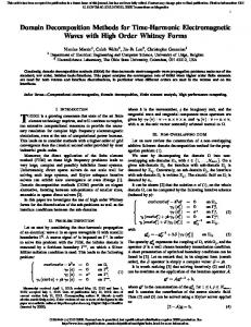
non interacting CPS beams can be identified with the same criteria discussed above; then, the relevant column of the transport matrix can be directly set to zero. Finally, the size of the linear system obtained by connecting all the subdomains is moderate, due to the reduced number of interacting wave objects. 6. THE SPECIAL CASE OF ITERATIVE PHYSICAL OPTICS In order to illustrate the potential of the method, we consider the special case of an iterative Physical Optics (PO) approach applied to separate objects. In this case, the proposed approach consists in constructing the individual GSM by PO, and provides the same results of an iterative PO, but with a big computational advantage. We analyze in particular the radiation of an elementary source in the presence of a number of square metallic plates. The simple example of a single 2λ × 2λ metallic plate illuminated by an elementary electric dipole is considered first. A spherical √ equivalence surface of radius γ = rmin + λ/10, (where rmin = 2λ is the radius of the minimum sphere enclosing the plate) has been defined for the plate. The number of CPS beams in the basis has been chosen according to Eq. (15) with χ ∼ = 1.5, NDOF = 2NSW (NSW + 2) and NSW = dkrmin e + 4[30], corresponding to N = 594. The imaginary part of the CPS locations has been taken equal to the real part b = γ. The scattering matrix for the metallic plate has been obtained through physical optics. Although the elementary source could be considered as a particular case of CPS itself, a CPS beam basis has been defined also for the source, consisting of 144 CPS located on a complex sphere of radius 0.7λ(1 − j). The elementary dipole is located at the origin of a rectangular coordinate system and polarized along √ z, the plate is centered at the point of coordinate (0, 3 3/2λ, 3/2λ) with the normal pointing towards the origin (plate 1 of Fig. 10(a)). Fig. 8(a) shows a comparison between the scattered electric field provided by this approach (solid line) and the one obtained by the electromagnetic software FEKO through a direct physical optics (PO) approach (circles). An excellent agreement is observed, which testifies that the proposed approach provides the same accuracy of the method used for the construction of the scattering matrix. A similar agreement is obtained for the phase. As a second step, another plate, identical to the √ first one, has been added, with its center located at the point (0, −3 3/2λ, 3/2λ) and the normal pointing towards the origin (plate 2 of Fig. 10(a)). It is worth noting that the GSM calculated for the previous example has been re-

30 Proposed approach FEKO (PO) 20 10 0 -10 z -20 -30 y -40 x -150 -100 -50 0 50 100 150 θ (deg)

465

FEKO (PO, sixth order) 30 Proposed approach 25 20 15 10 5 z 0 -5 x y -10 -150 -100 -50 0 50 100 150 θ (deg)

|E|θ (dB)

|E|θ (dB)

Progress In Electromagnetics Research B, Vol. 19, 2010

(a)

1

2

(b)

Figure 8. Electric field scattered by one (a) or two (b) metallic plates illuminated by an electric dipole. The geometry for the problem is shown in the inset. The scattered field is observed in the plane φ = 90◦ at a distance R = 10λ from the origin. In (b), the iterative PO results from FEKO are evaluated by considering reflections up to the sixth order. 0 100 200 300 400 500 0 100 200 300 400 500

Figure 9. Structure of the GTM T1,2 for the two plate configuration. used to study this new problem. Hence, no further PO calculations have been performed, but only a re-definition of the position and orientation of the ports. Fig. 8(b) compares the results provided by the CSP beam GSM approach (solid line) and those obtained with the software FEKO through an iterative PO approach considering multiple interactions up to the sixth order (circles). Also in this case the agreement is excellent. It is observed that, although the distance between the two plates is moderate, and the CPS beams used are not very directive, the generalized transport matrices are strongly sparse. The structure of the matrix T1,2 is illustrated in Fig. 9, where the black dots correspond to entries whose absolute value is greater than one thousandth of the largest element in the matrix; these entries are

466

Martini, Carli, and Maci z

1 2

3

y

x

(a) 30 25 20 |E|θ (dB)

15 10 5 0 -5 -10 -15

Proposed approach FEKO (PO, no mulitple reflections) FEKO (PO, second order) FEKO (PO, sixth order)

-150

-100

-50

0 θ (deg)

50

100

150

(b)

Figure 10. Scattering from 3 plates illuminated by an hertzian dipole. (a) Geometry for the problem and relevant subdomain numbering. (b) Scattered electric field in the plane φ = 90◦ at a distance R = 10λ from the origin. less then 4% of the total entries in the matrix. Empty columns in the figure correspond to CSP beams of the subdomain 2 which illuminate negligibly the subdomain 1. As a final example, the scattering from three plates has been analyzed. To this end, a third plate has been added, with its center located at the point (0, 0, −3λ) and the normal pointing towards the origin (plate 3 of Fig. 10(a)). The scattered field is shown in Fig. 10(b), where the proposed approach (continuous line) is compared with a direct PO approach not accounting for multiple reflections (asterisks), a direct PO approach considering also double reflections (dash-dotted line) and a direct PO approach accounting for up to six reflections (circles). As it is apparent, the results of the commercial software converge to the ones of the GSM-DD approach if an increasing number of reflections is accounted for. This demonstrates that the

Progress In Electromagnetics Research B, Vol. 19, 2010

467

proposed procedure correctly predicts the effects of all the multiple PO interactions. Indeed, no approximations are done in the connection step as long as the wave object basis is complete for the electric field representation. This means that if a full-wave method is used for the calculation of the sub-domain scattering matrices, the final accuracy is the same that would be obtained by analyzing the overall domain with the same technique. It is also noted that in all the examples the electric field is observed at a distance of 10λ from the origin. For the two and three plate cases this is in the near field zone of the overall scattering system, whose maximum linear dimension is greater than 6λ; the accuracy of the results demonstrates that the validity of the proposed procedure is not restricted to far-field calculation. Also for the threeplate configuration, the previously calculated GSM and impedance matrices were used for all the plates; hence, the solution of the problem only required the construction of the transport matrices, accounting for the plates position and orientation, and the solution of the global linear system, which is characterized by a strongly sparse system matrix. These steps required no more than a couple of minutes on a personal computer. On the other hand, the standard PO computation required some hours on the same computer. 7. CONCLUSION A Generalized Scattering Matrix Domain Decomposition Method using CPS beams as propagators has been proposed for an efficient description of the interactions in complex electromagnetic environments. The classical advantages of the DDM (possible reuse of the solutions, parallel solving capability, limited computational resource requirement) are combined with the benefits deriving from the angular selectivity of the complex point sources, that provide a substantial time saving in the construction and solution of the final linear system. The proposed approach presents the advantage of permitting the use of different methods for the calculation of the scattering from the various subdomains, thus, allowing the use of the most appropriate technique for the analysis of each subdomain. Furthermore, it becomes extremely efficient for problems of antenna installation or positioning, or for the analysis of structures containing geometrical repetitions, since the single scattering matrices can be reused in successive computations. Other interesting applications are concerned with iterative PO calculations, or the accurate characterization of quasi-optical beam waveguides, where the cascade of several electrically large reflectors has to be analyzed, and a multiple PO approach

468

Martini, Carli, and Maci

becomes prohibitively expensive. At present, only non intersecting subdomains delimited by spherical surfaces have been considered, which poses some limitations on the minimum distance between the different objects in the considered scenario. The approach can be extended to deal with subdomain boundaries conforming to the effective shape of the real source/scatterer, thus, relaxing the limitation on the mutual distance. Complete elimination of this impairment for treating overlapping domain is the objective of a future work. ACKNOWLEDGMENT This work was supported by IDS S.p.A., Pisa, Italy, under research contract STF/STAE 2007. APPENDIX A. CALCULATION OF THE GSM, THE GTM AND b(0) , A.1. The Impedance Matching Matrices The generic element Zij of a self-impedance matching matrix is obtained by projecting the field of the j-th CPS of the basis onto the i-th testing function, with basis and testing functions belonging to the same subdomain. For the external (internal) matching, the generic (n,n) entry Zi,j of the SMM (i = 1, . . . , Nn , j = 1, . . . , Nn ) is given by ³ ´ ³ ´ (n,n) (n) (n) (n) ˆ(n) = G s(n) − ˜ ˆ(n) · J ˆ(n) Zi,j = Ψj si ·J r ·J (A1) i i j j i (n)

(n)

(n)

(n)

with si ∈ Σext (si ∈ Σint ). For the mutual-impedance matching matrix, basis and testing functions belong to different subdomains and the generic entry (n,m) Zi,j , (i = 1, . . . , Nn , j = 1, . . . , Nm ) is given by ³ ´ ³ ´ (n,m) (m) (n) (m) ˆ(n) = G s(n) − ˜ ˆ(m) · J ˆ(n) Zi,j = Ψj si ·J r ·J (A2) i i j j i (n)

with si

(n)

∈ Σint .

A.2. The Primary Source Vector b(0) The primary source field is expanded in terms of CPS as in (1) N X (0) (0) E(0) (r) = bj Ψj (r). (A3) j=1

Progress In Electromagnetics Research B, Vol. 19, 2010

469 (0)

(0)

ˆ Taking the inner product with each testing functions δ(r − si )J i (0) defined on the external surface Σext leads to the equations (0)

E

(0) (si )

ˆ(0) = ·J i

N X

(0)

(0)

b j Ψj

³ ´ (0) ˆ(0) si ·J i

i = 1, . . . , N0

(A4)

j=1

which can be compactly rewritten as V(0) = Z(0,0) b(0) ,

(A5)

(0)

where b(0) = {bj } is the unknown source coefficient vector and V(0 = (0) ˆ(0) } is the excitation vector containing the tangential {E(0) (sj ) · J j components of the primary source electric field at the test points. The solution of the linear system in (A5) yields the required source coefficient vector. A.3. The GSM (n)

Let us assume that the sub-domain n is excited with a coefficient ap (n) (n) at the p-th port, i.e., it is illuminated by the field ap Ψp (r)), with all the other ports matched, namely anp0 = 0 for p0 6= p (this condition is automatically satisfied if the sub-domain n is isolated in free space). (n) (n) The field ap Ep (r) scattered by the subdomain constituents under this illumination is expanded in terms of outgoing CPS as N X

(n) a(n) p Ep (r) =

(n)

(n)

bj,p Ψj (r)

p = 1, . . . , Nn .

(A6)

j=1 (n)

Dividing both members of (A6) by ap E(n) p (r) =

N X

(n)

(n)

Sjp Ψj (r)

leads to p = 1, . . . , Nn

(A7)

j=1

(n)

where Sjp

¯ (n) (n) ¯ = bj,p /ap ¯

(n)

ap0 =0,p0 6=p

are the entries of the GSM and

(n)

Ep (r) is the field scattered by the subdomain n when it is illuminate (n) by the unit moment CPS Ψp (r). Taking the inner product with the (n) testing functions defined on an external spherical surface Σext leads to N ³ ´ ³ ´ X (n) (n) (n) (n) (n) ˆ ˆ(n) E(n) s · J = S Ψ s ·J p i i jp j i i j=1

i = 1, . . . , Nn . (A8)

470

Martini, Carli, and Maci

After repeating this procedure for all the CPS of the basis, Nn linear systems of the form in (A8) are obtained, which can be collected in the following matrix system W(n) = Z(n,n) S(n) ,

(A9)

(n) (n) ˆ(n) }i=1,...Nn , S(n) = {S (n) }j=1,...Nn , and where W(n) = {Ep (si ) · J i jp p=1,...Nn

p=1,...Nn

Z(n,n) is the SMM defined in (A1). The solution of this system provides the entries of the scattering matrix S(n) h i−1 S(n) = Z(n,n) W(n) . (A10) A.4. The GTM Let us assume that the sub-domain n is excited by the output of the q(m) th port of the subdomain m with a coefficient bq (i.e., it is illuminated (m) (m) by the field bq Ψq (r)) in the hypothesis that the subdomain m is isolated free space (i.e., the content of all the other subdomains is (n) removed). This field is expanded in series of CPS beams Ψp (r) of (n,m) the subdomain n with the unknown coefficients ap,q (m) b(m) q Ψq (r) =

N X

(n) a(n,m) p,q Ψp (r)

q = 1, . . . Nn .

(A11)

p=1 (n)

Dividing both members of (A6) by bq Ψ(m) q (r) =

N X

n,m (n) Tpq Ψp (r)

leads to q = 1, . . . Nn ,

(A12)

p=1

(n,m)

where Tpq

(n,m)

= ap,q

¯ (m) ¯ /bq ¯

(m)

bq0 =0,q 0 6=q

are the entries of the GTM.

Taking the inner product with the testing functions defined on an (n) internal spherical surface Σint leads to (n)

(n)

ˆ Ψ(m) q (si ) · Ji

=

N X

(n)

(n)

(n,m) ˆ . Tpq Ψp(n) (si ) · J i

(A13)

p=1

Repeating this procedure for all the CPS of the basis leads to Nm linear systems of the form in (A13), which can be collected in the following matrix system (A14) Z(n,m) = Z(n,n) T(n,m) ,

Progress In Electromagnetics Research B, Vol. 19, 2010

471

where Z(n,n) and Z(n,m) are defined in (A1) and (A2) respectively. The rectangular GTS is found by solving the system in (A14). This matrix is sparse if the two subdomains are not too close one to the other, due to the sparsity of Z(n,m) . We note that the calculation of T(n,m) requires the inversion of Z(n,n) , which has dimensions Nn × Nn . For a good choice of the CPS selectivity, this matrix is well-conditioned, and the inverse can be pre-calculated, stored and re-used in all the calculations relative to the subdomain n. The matrix system for the reciprocal transmission matrix from the sub-domain n to the subdomain m can be obtained by interchanging the indexes m and n in (A14). For the special case n = m, (A14) leads to T(n,n) = I, as expected. REFERENCES 1. Vouvakis, M., Z. Cendes, and J.-F. Lee, “A FEM domain decomposition method for photonic and electromagnetic band gap structures,” IEEE Transactions on Antennas and Propagation, Vol. 54, No. 2, 721–733, Feb. 2006. 2. Leopold, P. R., B. Felsen, and M. Mongiardo, “Electromagnetic field representations and computations in complex structures I: Complexity architecture and generalized network formulation,” International Journal of Numerical Modelling: Electronic Networks, Devices and Fields, Vol. 15, No. 1, 93–107, 2002. 3. Barka, A. and P. Caudrillier, “Domain decomposition method based on generalized scattering matrix for installed performance of antennas on aircraft,” IEEE Transactions on Antennas and Propagation, Vol. 55, No. 6, 1833–1842, Jun. 2007. 4. Van de Water, A. M., B. P. de Hon, M. C. van Beurden, A. G. Tijhuis, and P. de Maagt, “Linear embedding via Green’s operators: A modeling technique for finite electromagnetic bandgap structures,” Physical Review E (Statistical, Nonlinear, and Soft Matter Physics), Vol. 72, No. 5, 056704, 2005. 5. Li, M.-K. and W. C. Chew, “Wave-field interaction with complex structures using equivalence principle algorithm,” IEEE Transactions on Antennas and Propagation, Vol. 55, No. 1, 130– 138, Jan. 2007. 6. Nikolsky, V. V. and T. I. Nikolskaya, Decomposition Approach to the Problems of Electrodynamics, Nauka, National Bureau of Standards, Moscow, 1983. 7. Kerns, D. M., Plane-wave Scattering-matrix Theory of Antenna-

472

8.

9. 10. 11.

12.

13.

14.

15. 16.

17.

18.

Martini, Carli, and Maci

antenna Interactions, Tech. Rep. NBS Monograph 162, Nat. Bur. Stand., 1981. Elsherbeni, A. Z. and A. A. Kishk, “Modeling of cylindrical objects by circular dielectric and conducting cylinders,” IEEE Transactions on Antennas and Propagation, Vol. 40, 96–99, Jan. 1992. Felbacq, D., G. Tayeb, and D. Maystre, “Scattering by a random set of parallel cylinders,” Journal of the Optical Society of America A, Vol. 11, 2526–2538, Sep. 1994. Peterson, B. and S. Str¨om, “T matrix for electromagnetic scattering from an arbitrary number of scatterers and representations of E(3),” Phys. Rev. D, Vol. 8, No. 10, 3661–3678, Nov. 1973. Tsang, L., C. E. Mandt, and K. H. Ding, “Monte Carlo simulations of the extinction rate of dense media with randomly distributed dielectric spheres based on solution of Maxwell’s equations,” Optics Lett., Vol. 17, No. 5, 314–316, Mar. 1992. Yan, W.-Z., Y. Du, Z. Li, E. Chen, and J. Shi, “Characterization of the validity region of the extended T-matrix method for scattering from dielectric cylinders with finite length,” Progress In Electromagnetics Research, PIER 96, 309–328, 2009. Rubio, J., M. Gonzalez, and J. Zapata, “Generalized-scatteringmatrix analysis of a class of finite arrays of coupled antennas by using 3-D fem and spherical mode expansion,” IEEE Transactions on Antennas and Propagation, Vol. 53, No. 3, 1133–1144, Mar. 2005. Crocco, L., F. Cuomo, and T. Isernia, “Generalized scatteringmatrix method for the analysis of two-dimensional photonic bandgap devices,” J. Opt. Soc. Am. A, Vol. 24, No. 10, A12–A22, 2007. Felsen, L. B., “Complex source point solution of the field equations and their relation to the propagation and scattering of Gaussian beams,” Symposia Mathematica, Vol. 18, 39–56, 1976. Carli, G., E. Martini, and S. Maci, “Space decomposition method by using complex source expansion,” Proc. IEEE Antennas and Propagation Society International Symposium 2008, Jul. 1–4, 2008. Carli, G., E. Martini, M. Bandinelli, and S. Maci, “Domain decomposition and wave coupling by using complex source expansions,” Proc. 3rd European Conference on Antennas and Propagation, EuCAP 2009, 2079–2082, Mar. 2009. Tap, K., P. Pathak, and R. Burkholder, “Exact complex source

Progress In Electromagnetics Research B, Vol. 19, 2010

19. 20. 21.

22.

23. 24. 25. 26. 27.

28. 29. 30.

473

point beam expansion of electromagnetic fields from arbitrary closed surfaces,” Proc. IEEE Antennas and Propagation Society International Symposium 2007, 4028–4031, Jun. 2007. Tap, K., P. Pathak, and R. Burkholder, “An exact CSP beam representation for EM wave radiation,” International Conference on Electromagnetics in Advanced Applications, 75–78, Sep. 2007. Boag, A. and R. Mittra, “Complex multipole-beam approach to three-dimensional electromagnetic scattering problems,” J. Opt. Soc. Am. A, Vol. 11, No. 4, 1505–1512, 1994. Erez, E. and Y. Leviatan, “Electromagnetic scattering analysis using a model of dipoles located in complex space,” IEEE Transactions on Antennas and Propagation, Vol. 42, No. 12, 1620– 1624, Dec. 1994. Tap, K., P. Pathak, and R. Burkholder, “Fast complex source point expansion for accelerating the method of moments,” International Conference on Electromagnetics in Advanced Applications, 2007, ICEAA 2007, 986–989, Sep. 2007. Coifman, R., V. Rokhlin, and S. Wandzura, “The fast multipole method for the wave equation: A pedestrian prescription,” IEEE Antennas and Propagation Magazine, Vol. 35, 7–12, 1993. Pozar, M., Microwave Engineering, 2nd edition, Wiley, New York, 1998. Bucci, O. and G. Franceschetti, “On the degrees of freedom of scattered fields,” IEEE Transactions on Antennas and Propagation, Vol. 37, No. 7, 918–926, Jul. 1989. Bucci, O., “Computational complexity in the solution of large antenna and scattering problems,” Radio Sci., Vol. 40, 2005. Stupfel, B. and Y. Morel, “Singular value decomposition of the radiation operator application to model-order and far-field reduction,” IEEE Transactions on Antennas and Propagation, Vol. 56, No. 6, 1605–1615, Jun. 2008. Leopardi, P., “A partition of the unit sphere into regions of equal area and small diameter,” Electronic Transactions on Numerical Analysis, Vol. 25, 309–327, 2006. Martini, E., G. Carli, and S. Maci, “An equivalence theorem based on the use of electric currents radiating in free space,” Antennas and Wireless Propagation Letters, Vol. 11, 421–424, 2008. Hansen, J. E., Spherical Near-field Antenna Measurements, Peter Peregrinus Ltd., London, 1988.