A Semantic Text Retrieval for Indonesian using Tolerance ... - Lecturer

A Semantic Text Retrieval for Indonesian using Tolerance Rough Sets Models? Gloria Virginia** and Hung Son Nguyen*** **Duta Wacana Christian University, Informatics Engineering Department Dr. Wahidin Sudirohusodo 5-25, 55224 Yogyakarta, Indonesia ***University of Warsaw, Faculty of Mathematics, Informatics and Mechanics Banacha 2, 02-097 Warsaw, Poland

Abstract. The research of Tolerance Rough Sets Model (TRSM) ever conducted acted in accordance with the rational approach of AI perspective. This article, which was a doctoral thesis, presented studies who complied with the contrary path, i.e. a cognitive approach, for an objective of a modular framework of semantic text retrieval system based on TRSM specifically for Indonesian. In addition to the proposed framework, this thesis proposes three methods based on TRSM, which are the automatic tolerance value generator, thesaurus optimization, and lexicon-based document representation. All methods were developed by the use of our own corpus, namely ICL-corpus, and evaluated by employing an available Indonesian corpus, called Kompas-corpus. The endeavor of a semantic information retrieval system is the effort to retrieve information and not merely terms with similar meaning. This thesis is a baby step toward the objective. Keywords: Information retrieval, Tolerance rough sets model, text mining

1

Introduction

1.1

Information Retrieval

The percentage of individuals using the Internet continues to grow worldwide and in developing countries the numbers doubled between 2007 and 20111 . Accessing information by utilizing search systems becomes one habitual activity of million of people in facilitating their business, education, and entertainment in their daily life. The applications, such as web search engines which providing access to information over the Internet, are the most usual applications heavily use information retrieval (IR) service. Information retrieval is concerned with representing, searching, and manipulating large collections of electronic text and other human-language data [1, ?

1

This work was partially supported by the Polish National Science Centre grant 2012/05/B/ST6/03215 Key statistical highlights: ITU data release June 2012. URL: http://www.itu.int. Accessed on 25 October 2012.

2

G. Virginia and H. S. Nguyen

p. 2]. Clustering systems, categorization systems, summarization systems, information extraction systems, topic detection systems, question answering systems, and multimedia information retrieval systems are other applications utilize IR service. The main task of information retrieval is to retrieve relevant documents in response to a query [2, p. 85]. In a common search application, an ad hoc retrieval mode is applied in which a query is submitted (by a user) and then evaluated against a relatively static document collection. A set of query identifying the possible interest to the user may also be supplied in advanced and then evaluated against newly created or discovered documents. This operational mode where the queries remain relatively static is called filtering. Documents (i.e. electronic texts and other human-language data) are normally modeled based on the positive occurrence of words while the query is modeled based on the positive words of interest clearly specified. Both models then are examined in similarity basis using a devoted ranking algorithm and the output of information retrieval system (IRS) will be an ordered list of documents considered pertinent to the query at hand. In the keyword search technique commonly used, the similarity between documents and query is measured based on the occurrence of query words in the documents. Thus, if the query is given by a user, then the relevant documents are those who contain literally one or more words expressed by him/her. The fact is, text documents (and query) highly probable come up in the form of natural language. While human seems effortless to understand and construct sentences, which may consist of ambiguous or colloquial words, it becomes a big challenge for an IRS. The keyword search technique is lack of capability to capture the meaning of words, wherefore the meaning of sentences, semantically on documents and query because it represents the information content as a syntactical structure which is lack of semantical relationship. For example, a document contains words choir, performance, and ticket may talk about a choir concert, in spite of the fact that the word concert is never mentioned on that particular document. When a user inputs the word concert to define his/her information need, the IRS which approximate the documents and query in a set of occurrence words may deliver lots of irrelevant results instead of corresponding documents. We may expect better effectiveness to IRS by mimicking the human capability of language understanding. We should move from keyword to semantic search technique, hence the semantic IRS.

1.2

Philosophical Background

Semantic is the study of linguistic meaning [3, p. 1]. Sentence and word meaning can be analyzed in terms of what speakers (or utterers) mean of his/her utterances2 [4]. With regard to the intended IRS, we devoted our study to written 2

Utterances may include sound, marks, gesture, grunts, and groans (anything that can signal an intention)

A Semantic Text Retrieval for Indonesian using TRSM

3

document, which might be seen as an extension of speech. Hence, a text semantic retrieval system should know to some extent the meaning of words of texts being processed, so to speak. Intentionality Among others, Searl [5] and Grice [6] have been on a debate, namely the role of intentionality in the theory of meaning. Intentionality (in Latin: intendere; meaning aiming in a certain direction, directing thoughts to something, on the analogy to drawing a bow at a target) has been used to name the property of minds of having content, aboutness, being about something [7, p. 89]. Thus, mental states such as beliefs, fears, hopes, and desires are intentional because they are directed at an object. For example, if I have a belief, it must be a belief of something, or if I have a fear, it must be a fear of something. However, mental states such as undirected anxiety, depression and elation are not intentional because they are undirected at an object (e.g. I may anxious without being anxious about anything), but the directed cases (e.g. I am anxious about something) are intentional. In addition that intentional is directed, another important characteristic of intentional was proposed by Searl [5] that every intentional state consists of an intentional content in a psychological mode. The intentional content is a whole proposition which determines a set of condition of satisfaction and the psychological mode (e.g. belief, desire, promise) determines a direction of fit (i.e. mind-to-world or world-to-mind) of its propositional content. An example should make this clear: If I make an assertive utterance that ’it is raining’, then the content of my belief is ’it is raining’. So, the conditions of satisfaction are ’it is raining’, and not, for example, that the ground is wet or the water is falling out of the sky3 . And, in my assertive utterance, the psychological mode is a ’belief’ of the state in question, so the direction of fit is ’mind-to-world’4 . Further, Searl claimed [5, p. 19-21] that intentional contents do not determine their condition of satisfaction in isolation, rather they are internally related in a holistic way to: a) other intentional contents in the Network of intentional states; and b) a Background of nonrepresentational mental capacities. The following is Searl’s example to describe the role of Network: Suppose there is a man who forms the intention to run for the Presidency of the United States. In order that his desire be a desire to run for the Presidency he must have a whole lot of beliefs such as: the belief that the United States is a republic, that it has a presidential 3

4

The reason is, in the context of speech act, we do not concern about whether the belief of a speaker is true or not, rather we concern about the intention of speaker what he/she wants to represent by his/her utterance. Thus, it might be the case that a speaker represents his/her false belief as a true belief to the audience, e.g. a speaker utters ’it is raining’, while in fact ’it is a sunny day’. In other words, ’the mind to fit the world’. It is because a belief is like a statement, can be true or false; if the statement is false then it is the fault of the statement, not the world. The world-to-mind direction of fit is applied for the psychological mode such as desire or promise; if the promise is broken, it is the fault of the promiser.

4


system of government, that it has periodic elections, and so on. And he would normally desire that he receives the nomination of his party, that people work for his candidacy, that voters cast votes for him, and so on. So, in short, we can see that his intention ’refers’ to these other intentional states. The Background is the set of practice, skills, habits, and stance that enable intentional contents to work in various ways. Consider these sentences: ’Berto opened his book to page 37’ and ’The chairman opened the meeting’. The semantic content contributed by the word ’open’ is the same in each sentence, but we understand the sentences quite differently. It is because the differences in the Background of practice (and in the Network) produce different understanding of the same verb. Meaning Language is one of the vehicles of mental states, hence linguistic meaning is a form of derived intentionality. According to Searle, meaning is a notion that literally applies to sentences and speech acts. He mentioned that the problem of meaning in its most general form is the problem of how do we get from the physics to the semantics. For this purpose, there are two aspects to meaning intentions: a) the intention to represent; and b) the intention to communicate. Here, representing intention is prior to communication intention and the converse is not the case. Hence, we can intend to represent something without intending to communicate it, but we cannot intend to communicate something without intending to represent it before. So to speak, in order to inform anyone that ’it is raining’ we need to represent it in our mind that ’it is raining’ then utter it. Conversely, we cannot inform anyone anything, i.e. that ’it is raining’, when we do not make any representation of the state of affairs of the weather in our mind. For Grice, when a speaker mean something by an utterance, he/she intends to produce certain effects on his/her audience and intends the audience to recognize the intention behind the utterance. By this definition, it seems that Grice has overlooked the intention to represent and overemphasized the intention to communicate. However, a careful analyses showed that Grice’s account goes along with Searl’s account [8], i.e. representing intention is prior to communication intention. Moreover, Grice definition makes a point that a successful speech act is both meaningful and communicative, i.e. the audience understands nothing when the audience does not recognize the intention behind the utterance, which can be happen when the speaker makes an utterance without intending to mean anything or fails to communicate it. The Importance of Knowledge Based on Searl’s and Grice’s accounts, it should be clear that there is distinction between intentional content and the form of its externalization. To ask for the meaning is to ask for an intentional content that goes with the form of externalization [5]. It is maintained that for a successful speech act, a speaker normally


5

chooses an expression which is conventionally fixed, i.e. by the community at large, to convey a certain meaning. Thus, before the selection process of appropriate expressions, it is fundamental for a speaker to know about the expression in order to produce an utterance, and consequently the audience is required to be familiar with those conventional expressions in order to understand the utterance. We may infer now that Searl’s and Grice’s accounts pertaining the meaning suggest knowledge for language production and understanding. This knowledge should consists of concepts who are interrelated and commonly agreed by the community. The communication is satisfied when both sides are active participants and the audience experiences effects at some degree. 1.3

Challenges in Indonesian

Indonesian Studies Knowledge specifically for Indonesian is fundamental for a semantic retrieval system which processing Indonesian texts. The implication of this claim is far reaching, in particular because each language is unique. There are numerous aspects of monolingual text retrieval should be investigated for Indonesian, those including indexing and relevance assessment process, i.e. tasks such as tokenization, stopping, stemming, parsing, and similarity functions, are few to mention. Considerable effort with regard to information retrieval for Indonesian is showed by a research community in University of Indonesia (UI) since mid of 1990s. They reported [9] that their studies range in area of computational lexicography (i.e. creating dictionary and spell-checking), morphological analysis (i.e. creating stemming algorithms and parser), semantic and discourse analysis (i.e. based on lexical semantics and text semantic analysis), document summarization, question-answering, information extraction, cross language retrieval, and geographic information retrieval. Other significant studies conducted by Asian which proposed an effective techniques for Indonesian text retrieval [10] and published the first Indonesian testbed [11]. It is worth to mention that despite the long list of works ever mentioned, only limited number of the results is available publicly and among those Indonesian studies, it is hardly to find a work pertaining to automatic ontology constructor specifically. Indonesian Speakers The latest data released by Statistics Board of Indonesia (BPS-Statistics Indonesia)5 pertaining the population of Indonesia, showed that the number reached 237.6 million for the 2010 census. With the population growth rate 1.49 percent per year, the estimation of Indonesia population in 2012 is 245 million. This 5

BPS-Statistics Indonesia. URL: http://www.bps.go.id/. Accessed on 25 October 2012.

6


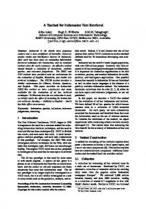
number ranked Indonesia on the forth most populous country in the world after China, India, and United States6 . The incredible number is not only related to the population. Indonesia, which is an archipelago country, has around 6,000 inhibited island over 17,5087 . Administratively, Indonesia consists of 33 provinces in which there are number of ethnics groups comes from each province which has its own regional language; according to Sneddon [12, p. 196], Indonesia has about 550 languages which is roughly one-tenth of all the languages in the world today. However, chosen as the national language, Bahasa Indonesia or Indonesian language is taught at all level of education and officially used in domains of formal activity, e.g. mass media, all government business, education, and law. Nowadays, most Indonesians are proficient in using the language; the number of speaker of Indonesian is approaching 100 percent [12, page 201]. Therefore, it is not overstated to consider Indonesian language as one of the large number of speakers in the world. Indonesian Internet Users Another significant challenge pertains to the growth of Internet users. As the global trend, the percentage of individuals using the Internet continues to grow worldwide and in developing countries the numbers doubled between 2007 and 20118 . For Indonesia, the Internet World Stats9 recorded that there are about 55 million internet users (with 22.4% penetration rate) and 43 million Facebook users (with 17.7% penetration rate) as of Dec. 31, 2011. Figure 1.1 shows the rapid growth of internet users in Indonesia during some previous years10 . These facts are some indicators of the digital media usage proliferation in Indonesia which is considered to keep on growing. 1.4

The Thesis

Tolerance Rough Sets Model Basically, an information retrieval system consists of three main tasks: (1) modeling the document; (2) modeling the query; and (3) measure the degree of correlation between document and query models. Thus, the endeavor of improving an IRS revolves around those three tasks. One of the effort is a method called tolerance rough set model (TRSM) which has performed positive results 6

7

8

9 10

July 2012 estimation of The World Factbook. URL: https://www.cia.gov. Accessed on 25 October 2012. Portal Nasional Indonesia (National Portal of Indonesia). URL: http://www. indonesia.go.id. Accessed on 25 October 2012. Key statistical highlights: International Telecommunication Union (ITU) data release June 2012. URL: http://www.itu.int. Accessed on 25 October 2012. URL: http://www.internetworldstats.com. Accessed on 25 October 2012. The graph was taken from the International Telecommunication Union (ITU). URL: http://www.itu.int/ITU-D/ict/statistics/explorer/index.html. Accessed on 25 October 2012.


7

Fig. 1.1: The growth of internet users in Indonesia. The figure shows the growth of internet users in Indonesia since 1990 to 2011. On 2011, the penetration rate was close to 18%.

on some studies pertaining to information retrieval. In spite of the fact that TRSM does not require complex linguistic process, it has not been investigated at large extent. Since it was formulated, tolerance rough sets model (TRSM) is accepted as a tool to model a document in a richer way than the base representation which is represented by a vector of TF*IDF-weight terms11 (let us call it TFIDFrepresentation). The richness of the document representation produced by applying the TRSM (let us call it TRSM-representation) is indicated by the number of index terms put into the model. That is to say, there are more terms belong to TRSM-representation than its base representation. The power of TRSM is grounded on the knowledge, i.e. thesaurus, which is comprised by index terms and the relationships between them. In TRSM, each set of terms considered as semantically related with a single term tj is called the tolerance class of a term Iθ (tj ), hence the thesaurus contains tolerance classes of all index terms. The semantic relatedness is signified by the terms co-occurrence in a corpus in which a tolerance value θ is set to define the threshold of cooccurrence frequency.

11

Appendix A provides an explanation about the TF*IDF weighting scheme.

8


1.5

Research Objective and Approach

The research aims to investigate the tolerance rough sets model in order to propose a framework for a semantic text retrieval system. The proposed framework is intended for Indonesian language specifically hence we are working with Indonesian corpora and applying tools for Indonesian, e.g. Indonesian stemmer, in all of the studies. The researches of TRSM ever conducted pertaining to information retrieval have focused on the system performance and involved a combination of mathematics and engineering in their studies [13–17]. In this thesis, we are trying to look at TRSM from a quite different viewpoint. We are going to do empirical studies involving observations and hypotheses of human behavior as well as experimental confirmation. According to the Artificial Intelligence (AI) view, our studies follow a human-centered approach, particularly the cognitive modeling12 , instead of the rationalist approach [19, p.1-2]. Analogous to two faces in a coin, both approaches would result in a comprehensive perspective of TRSM. In implementing the cognitive approach, we start our analysis from the performance of an ad hoc retrieval system. It is not our intention to compare TRSM with other methods and determine the best solution. Rather, we will take the benefit of the experimental data to learn and understand more about the process and characteristic of TRSM. The results of this process function as the guidance for computational modeling of some TRSM’s tasks and finally the framework of a semantic IRS with TRSM as its heart.

Thesis Structure Our research falls under the information retrieval umbrella. The following chapter provides an explanation about the main tasks of information retrieval and the semantic indexing in order to establish a general understanding of semantic IRS. Several questions are generated in order to assist us to scrutinize the TRSM. The issues behind the questions should be apparent when we proceed into the nature of TRSM that would be exposed on theoretical basis in Section 3. We have selected four subjects of question and will discuss them in the following order: 1. Is TRSM a viable alternative for a semantic IRS? The simplicity of characteristic and positive result of studies makes TRSM an intriguing method. However, before moving any further, we need to ensure that TRSM is reasonable to be the ground floor of the intended system. This issue will be the content of Section 4. 12

The cognitive modeling is an approach employed in the Cognitive Science (CS). Cognitive science is an interdisciplinary study of mental representations and computations and of the physical systems that support those processes [18, p.xv].


9

2. How to generate the system knowledge automatically? The richer representation of document yielded by TRSM is achieved fundamentally by means of a knowledge, which is a thesaurus. The thesaurus is manually created, in the sense that a parameter, namely tolerance value θ, is required to be determined by hand. In Section 5 we would propose an algorithm to resolve the matter in question, i.e. to select a value for θ automatically. 3. How to improve the quality of the thesaurus? The thesaurus of TRSM is generated based on a collection of text documents functions as a data source. In other words, the quality of document representation should depend on the quality of data source at some degree. Speaking of which, the TRSM basically works based on the co-occurrence data, i.e. the raw frequency of terms co-occurrence, and it arises an assumption that other co-occurrence data might bring a benefit for the effort to optimize the thesaurus. These presumptions would be reviewed and discussed in Section 6. 4. How to improve the efficiency of the intended system? The TRSM-representation is claimed to be richer in the sense that it consists of more terms than the base representation. Despite the fact that the terms of TRSM-representation are semantically related, more terms on document vector results in more cost of computation. In other words, system efficiency becomes the trade-off. We came into an idea of a compact document representation that would be explained in Section 7. This thesis proposes three methods based on TRSM for the mentioned problems. All methods, which are discussed in Section 5 to 7, were developed by the use of our own corpus, namely ICL-corpus, and evaluated by employing an available Indonesian corpus, called Kompas-corpus13 ; Section 8 describes the evaluation process. The evaluation on the methods achieved satisfactory results, except for the compact document representation method; this last method seems to work only in limited domain. The final chapter provides our conclusion of the research as well as discussion of some challenges that lead to advance studies in the future. Contribution The main contribution of this thesis is the modular framework of text retrieval system based on TRSM for Indonesian. Pertaining to the framework, we introduced novel strategies, which are the automatic tolerance value generator, thesaurus optimization, and lexicon-based document representation. An other contribution is a new Indonesian corpus (ICL-corpus), accompanied by a corpus consists of keywords defined by human experts (WORDS-corpus), in which both follow the format of Text REtrieval Conference (TREC)14 [20] and ready to be 13 14

Explanation about all corpora used in this thesis is available in Appendix C. TREC is a forum for IR community which provides an infrastructure necessary to evaluate an IR system on a broad range of problems. URL: http://trec.nist.gov/.

10


used for an ad hoc evaluation of IRS. These contributions should open wider research directions pertinent to information retrieval.

2

Semantic Information Retrieval

2.1

Information Retrieval Models

The main problem of information retrieval system is the issue of determining the relevancy of a document with regard to the information need. The decision whether documents are relevant or not relies on the ranking algorithm being used which plays the role of calculating the degree of association between documents and the query as well as defining the order of documents by its degree of association, in which the top documents are considered as the most relevant ones. In order to work, a ranking algorithm considers fundamental premises which are a set of representations of documents in given collection D, a set of representations for user information needs (user queries) Q, and a framework for modeling document/query representation F. These basic premises, together with the ranking function R, determines the IR model as a quadruple [D, Q, F, R] [21, p. 23]. Baeza-Yates and Ribeiro-Neto [21] structured 15 IR models covered in their book into a taxonomy as well as discussed them theoretically and bibliographically. Figure 2.1 presents the summary of the taxonomy. A clear distinction is made on the way a user pursues information: by searching or by browsing. While browsing, a user might explore a document space which is constructed in a flat, hierarchical, or navigational organization. Another user might prefer to submit a query to the system and put the burden of searching process to the system. In order to accomplish the task, the system could analyze each document by reference to the document’s content only or combination between the content and the structure of document. The structured model considers the latter while the classic model focusses on the former. The classic model is differentiated into three models with regard to the document representation: boolean, vector, and probabilistic. Respectively, in Boolean and probabilistic models, a document is represented based on set theory and probability theory, while vector model will represent a document as a vector in a high-dimensional space. In this thesis, we apply the classic vector model where document and query are represented as vectors in a high-dimensional space and each vector corresponds to a term in the vocabulary of the collection. The framework then is composed of a high-dimensional vectorial space and the standard linear algebra operations on vectors. The association degree of documents with regard to the query is quantified by the cosine of the angle between these two vectors15 . 2.2

The Main Tasks of Information Retrieval

Suppose each text document conveys meaning expressed in the form of written words chosen specifically and subjectively by the writer. When text documents 15

Appendix B provides explanation about Cosine similarity measure as a document ranking algorithm.


11

Fig. 2.1: A taxonomy of IR models. A summary of the IR models taxonomy structured by Baeza-Yates and Ribeiro-Neto.

are fed into an IRS who employs vector space model, the text documents would be transformed into vectors of a space whose dimension is consistent with the number of index terms in the corpus. A query which conveys information need of a user could be considered as a pseudo-document, thereby analogous scenario and activities occur at user side. In the searching process, a ranking algorithm works over these two representations by measuring the degree of correlation between them. By reference to its process, IR consists of three main tasks which are figured in Fig. 2.2 as filled rectangles: document modeling, query modeling, and matching process. The figure reflects that a successful matching process has two requirements: (1) models common to both query and document; and (2) system capability to construct a model which represent the information need of the user as well as the content of text document.

Fig. 2.2: The main tasks of information retrieval. Information retrieval consists of three tasks: (1) document modeling; (2) query modeling; and (3) matching process.

Explained in the previous chapter, Searl’s and Grice’s accounts on meaning suggest knowledge shared by the speaker and its audience (i.e. the user and

12


the system) for a successful communication. Suppose the IRS has knowledge corresponding at some degree to human, still the distinction between intentional content and the form of its externalization rises some complexity for IRS in order to construct representations of user’s information need (in the query) and of author’s idea (in the document). Language production and understanding are capabilities of most human, achieved through learning activities during his/her life and supported by the biologically mechanism genetically endowed [22], while none of those capabilities and support possessed by a computer system naturally. Reduced meaning retained by the representations of user’s information need and of document’s content become the consequence. It is highly probable that user’s satisfaction of proper information with regard to his/her need then is sacrificed. 2.3

Semantic Indexing

Indexing is a process to construct a data structure over the text to speed up searching [21, p. 191]. The major data structure in IRS is inverted index (or inverted file) which provides a mapping between terms and their locations of occurrence in a text collection [1, p. 33]. The first paragraph of this chapter explained that in order to construct a model of IR, the representation of document (i.e. document indexing) as well as query should be first resolved before specifying the framework; and with these basis, an appropriate ranking function is determined. For a semantic IRS, shifting from traditional indexing into the semantic indexing hence becomes the first consideration. In case that the conventional retrieval strategies employ the bag-of-words representation of document and match directly on keywords, then the semantic indexing requires an enrichment of representation such that the IRS works with bag-of-concepts representation of documents and computes the concept similarity. Several techniques function for enrichment of document representation are latent semantic indexing (LSI), explicit semantic analysis (ESA), and extended tolerance rough sets model (extended TRSM). These three techniques apply the classic vector space model (VSM) and thus it is possible to use conventional metrics (e.g. Cosine) in matching task. Further, they do not rely on any humanorganized knowledge. LSI, ESA, and extended TRSM naturally use statistical co-occurrence data in order to enrich the document representation, however LSI works by applying singular value decomposition (SVD), ESA relies on knowledge repository (e.g. Wikipedia), and the extended TRSM is based on rough sets theory. As a technique to dimensionality reduction, LSI identifies a number of most prominent dimensions in the data, perceived as the latent concepts since these concepts cannot be mapped into the natural concepts manipulated by humans or the concepts generated by system. An opposite condition happens for ESA and extended TRSM, thus the entries of their vectors are explicit concepts. The following sections will describe LSI, ESA, and extended TRSM in the order given. For convenience of the explanation, a matrix is used as data structure where each entry defines the association strength between document and term.


13

The most common measure used to calculate the strength value is the TF*IDF weighting scheme defined in Equation (A.1). Latent Semantic Indexing Latent semantic indexing introduced by Furnas et al. [23] employs singular value decomposition (SVD) in 1988. By running SVD, it approximates the termdocument matrix into a lower dimensional space hence removes some of the noise found in the document and locates two documents with similar semantic (whether or not they have matching terms) close to one another in a multidimensional space [24]. Running the SVD means that a term-document matrix A is decomposed into the product of three other matrices such that T Am×n = Um×s Ds×s Vs×n .

(2.1)

Matrix U is the left singular vectors matrix whose columns are eigenvectors of the AAT and holds the coordinates of term vectors. Matrix V is the right singular vectors matrix whose columns are eigenvectors of the AT A and holds the coordinates of document vectors. Matrix D refers to a diagonal matrix whose elements are the singular values of A, sorted by magnitude. m is the total number of terms, n is the total number of documents, and s = min(m, n). The latent semantic representation of A is developed by keeping the top k singular values of D along with their corresponding columns in U and V T matrices. The result is a k-rank matrix A0 which is closest in the least squares sense to matrix A; it contains less noisy dimensions and captures the major associational structure of the data [23]. Figure 2.3 presents the schematic of SVD for matrix A and its reduced model. With regard to a query, its vector q is treated similar to matrix A by following this rule −1 T q1×k = q1×m Um×k Sk×k . (2.2) After all, the matching process between query and documents is conducted by computing the similarity coefficient between k-rank query vector qk and corresponding columns of k-rank matrix Vk . Explicit Semantic Analysis In 2007, Gabrilovich and Markovitch introduced the notion of explicit semantic analysis (ESA) [25]. Later, Gottron et al. [26] showed that ESA is a variation of the generalized vector space model (GVSM)16 [27] who considers term correlation. ESA represents documents and query as vectors in a high dimensional of concept space, instead of term space, thus each dimension corresponds to a concept. 16

Consistent with VSM, GVSM interprets index term vectors as linearly independent, however they are not orthogonal.

14


Fig. 2.3: The illustration of SVD. SVD illustration of a terms-by-documents matrix A of rank k.

Each coordinate of concept vector expresses the degree of association between the document and the corresponding concept. Suppose D = {d1 , . . . , di , . . . , dN } is a set of documents and T = {t1 , . . . , tj , . . . , tM } is the vocabulary of terms, then the association value uik between document di and concept ck , k ∈ {1, . . . , K} is defined as X uik = wij × cjk (2.3) tj ∈T

where wij denotes the weight of term tj in document di and cjk signifies the correlation between term tj and concept ck . Equation (2.3) describes the association value as the product of weight of term in document (wij ) and weight of concept in knowledge base concept (cjk ), hence there are two computations need to be done in advance. Basically, both computations could be done using the TF*IDF weighting scheme, however the former is calculated over a corpus functioned as the system data, while the latter is calculated over a corpus functioned as the knowledge base; thus there are two corpora functioned differently. The merge of system data’s and knowledge base’s weights yields a new representation for the system data, i.e. bag-of-concepts representation. Gabrilovich and Markovitch [25] suggests Wikipedia articles for the corpus functioned as the knowledge base considering that it is a vast amount of highly organized human knowledge and undergoes constant development. However, the main reason is Wikipedia treats each description as a separate article, thus each description is perceived as a single concept. By this definition, any collection of documents is possible to be used as the external knowledge base.


15

Fig. 2.4: The ESA. Visualization of the semantic indexing process in ESA.

Figure 2.4 shows the computation process of ESA in order to convert the bagof-words representation of system data into the bag-of-concepts representation by utilizing natural language definition of concepts from the knowledge base. Extended Tolerance Rough Sets Model As its name, the extended TRSM is an extension of TRSM proposed by Nguyen et al. [28] in 2012. Detail explanation about TRSM is available in the following chapter, hence in this section we focus only on the extension part of TRSM. The study of Nguyen et al. [28, 29] aimed to enrich the document representation worked in clustering task by incorporating other information than the index terms of document corpus, namely citation and semantic concept. The citation referred to the bibliography of a given scientific article while the semantic concept was constructed based on an additional knowledge source, i.e. DBpedia. Thereby, the extended TRSM was defined as a tuple RF inal = (RT , RB , RC , αn )

(2.4)

where RT , RB , and RC denote the tolerance spaces which are determined respectively over the set of terms T , the set of bibliography items cited by a document B, and the set of concepts in the knowledge domain C. The function αn : P (T ) −→ P (C) is called the semantic association for terms, thus αn (Ti ) is the set of n concepts most associated with Ti for any Ti ⊂ T [30].

16


In this model, each document di ∈ D associated with a pair (Ti , Bi ) is represented by a triple UR (di ) = {URT (di ), URB (di ), αn (Ti )}

(2.5)

where Ti is the set of terms occurring in document di and Bi is the set of bibliography items cited by document di . The study of extended TRSM which presented with positive results indicated that the method would be effective to be realized in a real application. It is obvious from Equation (2.4) and (2.5) that the extended TRSM accommodates different factors at once for a semantic indexing, instead of one factor such as in original TRSM as well as LSI and ESA. Further, the model is more nature considering the real life situation of information retrieval process.

3 3.1

Tolerance Rough Sets Model Rough Sets Theory

In 1982, Pawlak introduced a method called rough sets theory [31] as a tool for data analysis and classification. During the years, this method has been studied and implemented successfully in numerous areas of real-life applications [32]. Basically, rough sets theory is a mathematical approach to vagueness which expresses the vagueness of a concept by means of the boundary region of a set; when the boundary region is empty, it is a crisp set. Otherwise, it is a rough set [33]. The central point of rough sets theory is an idea that any concept can be approximated by its lower and upper approximations, and the vagueness of concept is defined by the region between its upper and lower approximations. Consider Fig. 3.1 for illustration.

Fig. 3.1: Rough Sets. Basic idea of rough sets theory as it is explained in [33]

Let us think of a concept as a subset X of a universe U , X ⊆ U , then in a given approximation space A = (U, R) we can denote the lower approximation


17

of concept X as LA (X) and the upper approximations of concept X as UA (X). The boundary region, BNA (X), is the difference between the upper and lower approximations, hence BNA (X) = UA (X) − LA (X)

(3.1)

Let R ⊆ U × U be an equivalence relation that will partition the universe into equivalence classes, or granules of knowledge, thus formal definition of lower and upper approximations are [ LA (X) = {R (x) : R (x) ⊆ X} (3.2) x∈U

UA (X) =

[

{R (x) : R (x) ∩ X 6= ∅}

(3.3)

x∈U

3.2

Tolerance Rough Sets Model

The equivalence relation R ⊆ U × U of classical rough sets theory required three properties [32]: reflexive (xRx), symmetric (xRy → yRx), and transitive (xRy ∧ yRz → xRz); for ∀x, y, z ∈ U , thus the universe of an object would be divided into disjoint classes. These requirements have been showed to be not suitable for some practical applications (viz. working on text data), because the association between terms was better viewed as overlapping classes (see Fig. 3.2), particularly when term co-occurrence was used to identify the semantic relatedness between terms [14] .

Fig. 3.2: Overlapping classes. Overlapping classes between terms root, basis, and cause [14]

The overlapping classes can be generated by a relation called tolerance relation which was introduced by Skowron and Stepaniuk [34] as a relation in generalized approximation space. The generalized approximation space is denoted as a

18


quadruple A = (U, I, ν, P ), where U is a non-empty universe of objects, I is the uncertainty function, ν is the vague inclusion function, and P is the structurality function. Tolerance Rough Sets Model (TRSM) was introduced by Kawasaki, Nguyen, and Ho in 2000 [13] as a document representation model based on generalized approximation space. In the information retrieval context, we can assume a document as a concept. Thus, implementing TRSM means that we approximate concepts determined over the set of terms T on a tolerance approximation space R = (T, I, ν, P ) by employing the tolerance relation. In order to generate the document representation, which is claimed to be richer in terms of semantic relatedness, the TRSM needs to create tolerance classes of terms and approximations of subsets of documents. If D = {d1 , d2 , ..., dN } is a set of text documents and T = {t1 , t2 , ..., tM } is a set of index terms from D, then the tolerance classes of terms in T is created based on the co-occurrence of index terms in all documents D. A document representation is represented as a vector of weight di = {wi,1 , wi,2 , ..., wi,M }, where wi,j denotes the weight of term tj in document di and calculated by considering the upper approximation of document di . Tolerance Approximation Space The definitions of tolerance approximation space R = (T, I, ν, P ) are as follows Universe: The universe U is the set of index terms T U = {t1 , t2 , ..., tM } = T

(3.4)

Tolerance class: Skowron and Stepaniuk [34] maintain that an uncertainty function I : U → P(U ), where P(U ) is a power set of U , is any function from U into P(U ) satisfying the conditions x ∈ I(x) for x ∈ U and y ∈ I(x) ⇔ x ∈ I(y) for any x, y ∈ U . This means that we assume the relation xIy ⇔ y ∈ I(x) is a tolerance relation and I(x) is a tolerance class of x. The parameterized tolerance class Iθ is then defined as Iθ (ti ) = {tj | fD (ti , tj ) ≥ θ} ∪ {ti }

(3.5)

where θ is a positive parameter and fD (ti , tj ) denotes the number of documents in D that contain both terms ti and tj . From Equation (3.5), it is clear that it satisfies the condition of being reflexive (ti ∈ Iθ (ti )) and symmetric (tj ∈ Iθ (ti )) required by a tolerance relation; the tolerance relation R ⊆ T × T can be defined by means of function Iθ as ti Rtj ⇔ tj ∈ Iθ (ti ). Assuming that a term is a concept, then the tolerance class Iθ (ti ) consists of terms related to a concept ti and the precision of the concept determined might be tuned by varying the threshold θ. Vague inclusion function: the vague inclusion function ν : P(U ) × P(U ) → [0, 1] measures the degree of inclusion between two sets and is defined as ν (X, Y ) =

|X ∩ Y | |X|

(3.6)


19

where the function ν must be monotone w.r.t the second argument, i.e. if Y ⊆ Z then ν(X, Y ) ≤ ν(X, Z) for X, Y, Z ⊆ U . Hence, the vague inclusion function can determine the matter whether the tolerance class I (x) of an object x ∈ U is included in a set X. Together with the uncertainty function I, the vague inclusion function ν defines the rough membership function for x ∈ U, X ⊆ U as µI,ν (x, X) = ν(I(x), X). Therefore, the membership function µ for ti ∈ T, X ⊆ T is defined as |Iθ (ti ) ∩ X| (3.7) µ (ti , X) = ν (Iθ (ti ) , X) = |Iθ (ti )| Structurality function: with structurality function P : I(U ) → {0, 1}, where I(U ) = {I (x) : x ∈ U }, one can construct two subsets based on value of P (I (x)), named structural subset and nonstructural subset, when P (I (x)) = 1 and P (I (x)) = 0 respectively. In TRSM, all tolerance classes of index terms are considered as structural subsets, hence for all ti ∈ T P (Iθ (ti )) = 1

(3.8)

Approximations With the foregoing definitions, we can define the lower approximation LR (X), upper approximation UR (X), and boundary region BNR (X) of any subset X ⊆ T in a tolerance space R = (T, Iθ , ν, P ) as follows LR (X) = {ti ∈ T | ν(Iθ (ti ), X) = 1}

(3.9)

UR (X) = {ti ∈ T | ν(Iθ (ti ), X) > 0}

(3.10)

BNR (X) = UR (X) − LR (X)

(3.11)

Refers to the basic idea of rough sets theory [33], for any set of X, intuitively we may assume the upper approximation as the set of concepts that share some semantic meanings with X, the lower approximation as the core concepts of X, while the boundary region consists of concepts that cannot be classified uniquely to the set or its complement, by employing available knowledge. TRSM Document Representation After all, the richer representation of document di ∈ D is achieved by simply representing the document with its upper approximation, i.e. UR (di ) = {ti ∈ T | ν(Iθ (ti ), di ) > 0} followed by calculating the weight vector using the i.e.   (1 + log fdi (tj )) log fDN(tj )    1 0 ∗ wij = log f N S (t )   mintk ∈di wik 1+log D Nj fD (tj )

(3.12)

extended weighting scheme, if tj ∈ di if tj ∈ / UR (di ) otherwise

(3.13)

20


where S is a normalisation factor applied to all document vectors. The extended weighting scheme is defined from the standard TF*IDF weighting scheme and is necessary in order to ensures that each term occurring in the upper approximation of di but not in the di itself has a weight smaller that the weight of any terms in di . By employing TRSM, the final document representation has less zero-valued similarities. This leads to a higher possibility of two documents having non-zero similarities although they do not share any terms. This is the main advantage the TRSM-based algorithm claims to have over traditional approaches. 3.3

The Challenges of TRSM

We identified that there are three fundamental components of TRSM to work which are dependent in sequence: (1) the tolerance classes of all index terms; (2) the upper document representation; and (3) the TRSM weighting scheme. Figure 3.3 displays the basic process of tolerance rough sets model which contains those three components.

Fig. 3.3: Tolerance rough sets model. The process of tolerance rough sets model.

A document representation based on TRSM (TRSM-representation) can be seen as the revised version of a base representation which is recalculated using the TRSM weighting scheme. The base representation is modeled by calculating the term frequency (TF) and the inverse document frequency (IDF) of a term, i.e. commonly called TF*IDF weighting scheme; hence we dub this representation the TFIDF-representation. Suppose the representation of document produced by TRSM and TF*IDF are structured as matrices, thus Figure 3.4 shows the relationship between them, where tf idf and trsm denote the weight of term computed by TF*IDF and TRSM weighting scheme respectively. During term weight computation, TRSM consults the upper document representation, whereas the upper representation of a document is only possible to be generated when the tolerance classes of all index terms are available. Refer


21

Fig. 3.4: Relationship between TFIDF-representation and TRSM-representation. The TRSM-representation is possible to be constructed by taking TFIDF-representation as the input of TRSM.

to Equation (3.5), a tolerance class of a term ti consists of all index terms consider as semantically related with the term ti and the precision of relatedness between a pair of terms is defined by the tolerance value θ. In other words, the importance of relationship between terms is determined by θ value. Based on the nature of TRSM, tolerance classes can be categorized as a thesaurus; a lightweight ontology who reflects the relationship between terms [35]. As the heart of TRSM, thesaurus becomes the knowledge of the system who implements it. It should be clear that in TRSM the quality of document modeling would rely on the thesaurus, and the quality of the thesaurus might depend on the tolerance value θ. Despite the fact that tolerance value is a critical element in TRSM, there is no formal mechanism available for its determination and it is a common practice that the selection is performed manually by the practitioners with regard to their data. This particular issue will be further discussed in Section 5. The thesaurus might be constructed based on an algorithm explained by Nguyen and Ho [15]. The algorithm takes a document-by-term matrix (i.e. the TFIDF matrix) as the input and yields the tolerance matrix, which is structured as a binary term-by-term matrix. Figure 3.5 shows the steps of the algorithm. Subsequently, the occurrence binary matrix OC matrix, the co-occurrence matrix COC matrix, and the tolerance matrix TOL matrix were generated in sequence manner by employing Equation (3.14), Equation (3.15), and Equation (3.16). Note that tf idfi,j denotes the weight of term j computed by TF*IDF scheme in document i, card(OC x AND OC y ) denotes the cardinality of two terms, tx and ty , being occurred together in a collection, and θ is the co-occurrence threshold of terms. oci,j = 1

⇔

tf idfi,j > 0 .

cocx,y = card(OC x AND OC y ) . tolx,y = 1

⇔

cocx,y ≥ θ .

(3.14) (3.15) (3.16)

In addition to tolerance value, the algorithm demonstrated that a data source might have an impact on the thesaurus quality since it manipulates a set of

22


Fig. 3.5: Relationship between TFIDF-representation and TRSM-representation. The TRSM-representation is possible to be constructed by taking TFIDF-representation as the input of TRSM.

documents functions as the only input. The effects might be as a consequence of the type of data source or the size of the collection. Another important subjects relevant to the thesaurus of TRSM is pertaining to the fact that the thesaurus is created based on the quantity of two terms occur together, thereby employs tolerance value θ as the threshold of semantic relatedness. In fact, refer to the term weighting scheme, there are other alternatives of co-occurrence data who takes more factors into consideration, e.g. the TF*IDF weighting scheme. By that means, other similarity measures, i.e. cosine, might be applied. The presumptions pertaining to thesaurus optimization will be examined in Section 6. Refer to the path of TRSM, its computation complexity is the aggregation of each task, i.e. thesaurus construction, upper representation generation, and re-weighting task. The first task requires O(N M ) [15], where N defines the number of documents and M defines the number of index terms, while the second and third tasks both require O(M 2 ). Thus totally, the upper bound of TRSM implementation would be O(N M 2 ). With regard to the system efficiency, minimizing the dimensionality of document vectors would be a practical alternative for the complexity. Using this as the starting point, in Section 7 we are going to introduce a novel model of document namely the lexicon-based representation.


4

23

The Potential of TRSM

4.1

Introduction

We may find studies showing the positive results of TRSM implementation for document clustering task [13–16], query expansion [17], and document retrieval task [36]. Those studies claimed that TRSM-representation was richer than the baseline representation (TFIDF-representation), however none has shown and explained empirically the richness. It has been known that the richness of TRSM-representation is understood as having less zero-value similarities and having higher possibility that two documents holding non-zero similarities although they do not share any terms. The result of our study presented in this chapter confirmed those affirmations and add another fact. We found that the TRSM-representation consists of terms considered as important by human experts. Further, the study revealed that rough sets theory seems to work in accordance with the natural way of human thinking. Finally, the study showed that TRSM is a viable option for a semantic IRS. 4.2

Experiment Process

We used two corpora, ICL-corpus and WORDS-corpus17 , with 127 topics. We took an assumption that each topic given by human experts in annotation process was a concept, therefore we considered the keywords determined by the human experts18 as the term variants that highly related with particular concept. These keywords are the content of text body in WORDS-corpus, hence each document of WORDS-corpus contains important terms of particular concept(s) selected by human experts. With regard to the automatic process of the system, we considered these keywords as the relevant terms for each document (which bear one or more topics) that should be selected by the system. Therefore, WORDS-corpus was treated as the ground truth of this study. Figure 4.1 shows the general process of the study and the dashed rectangle identifies the focus of the experiment, which were performed twice, i.e. with stemming task and without stemming task. Extraction Phase. The main objective of extraction phase was preprocessing both corpora. Confix-Stripping stemmer (CS stemmer), a version of Indonesian stemmer, was employed in the stemming task while Vega’s stopword [37] was applied in the stopword task19 . CS stemmer was introduced as a new 17

18

19

ICL-corpus consists of 1,000 documents taken from an Indonesian choral mailing list, while WORDS-corpus consists of 1,000 documents created from ICL-corpus in an annotation process conducted by human experts. Further explanation of these corpora is available in Appendix C.1. We collaborated with 3 choral experts during annotation process. Their backgrounds could be reviewed in Appendix C.3. We used CS stemmer and Vega’s stopword in all of our studies presented in this thesis.

24


Fig. 4.1: Main phases of the study. There were 3 main phases: extraction, rough sets, and analysis. A rectangle represents a process while a circle represent a result.

confix-stripping approach for automatic Indonesian stemming and was showed as the most accurate stemmer among other automated Indonesian stemmers [38]. Vega’s stopword has shown to produce the highest precision@10, R-precision, and recall values (although the differences without stopping words are not significant (p < 0.05), except for the recall value (0.038)), among other available Indonesian stopword lists [10]. Documents were tokenized based on character other than alphabetic. The resulted tokens were stemmed by the CS stemmer and then compared to the Vega’s stopword. It yielded lists of unique terms and its frequency. There were 9,458 unique terms extracted from ICL-corpus and 3,390 unique terms extracted from WORDS-corpus; called ICL list and WORDS list respectively. When it was run without stemming process, we identified 12,363 unique terms in ICL list and 4,281 unique terms in WORDS list. Both corpora were classified based on 127 topics yielded in preliminary process, i.e. annotation process20 . Recall that we took an assumption that each topic was a concept and keywords determined by human experts were important variants of a concept hence aggregation of terms appeared in each class were taken as the terms for representative vector of each class. The set of classes resulted from ICL-corpus was called IL while the set of classes resulted from WORDS-corpus was called WL; each set of class, IL and WL, consists of 127 classes. So, technically speaking, instead of document-term matrix, we worked with topic-by-term matrix.

Rough Set Phase. This phase was conducted in order to generate the lower set, upper set, and boundary set of each class in IL. These sets were possible to be created using Equation (3.9), Equation (3.10), and Equation (3.11) when tolerance classes of all index terms were ready. 20

Please see Appendix C.1 for explanation of annotation process.


25

The tolerance classes was constructed by following the steps described in Fig. 3.5 of previous chapter, with an exception that in this experiment the algorithm took the topic-by-term frequency matrix as its input. Thereby, Fig. 4.2 displays the steps applied for the thesaurus generation of this particular study.

Fig. 4.2: Tolerance classes construction. The construction of tolerance classes in this study took topic-term matrix as the input and produced a term-by-term matrix as the output. Here, M denotes the number of index term and N denotes the number of topic.

Analysis Phase. In analysis phase, we examined the mean recall and precision of upper set (US), lower set (LS), and boundary set (BS) of IL by taking the WL as the ground truth. The computations were run for co-occurrence threshold θ between 1 to 75. Recall and precision are the most frequent and basic measures for information retrieval effectiveness [39]. Recall R is the fraction of relevant documents that are retrieved while precision P is the fraction of retrieved documents that are relevant. Suppose Rel denotes relevant documents and Ret denotes retrieved documents, then recall R and precision P are defined as follows R=

](relevant items retrieved) |Rel ∩ Ret| = ](relevant items) |Rel|

(4.1)

](relevant items retrieved) |Rel ∩ Ret| = (4.2) ](retrieved items) |Ret| In this study, both measures were used for the terms rather than documents. That is to say, by considering WORDS list as the ground truth, then recall P =

26

G. Virginia and H. S. Nguyen Table 4.1: Formulas for recall and precision calculations. US

LS

BS

RecallW L

|W L ∩ U SIL | |W L ∩ LSIL | |W L ∩ BSIL | |W L| |W L| |W L|

PrecisionW L

|W L ∩ U SIL | |W L ∩ LSIL | |W L ∩ BSIL | |U SIL | |LSIL | |BSIL |

RecallIL

|IL ∩ U SIL | |IL|

|IL ∩ LSIL | |IL|

|IL ∩ BSIL | |IL|

R is the fraction of relevant terms that are retrieved while precision P is the fraction of retrieved terms that are relevant. The formulas applied for recall and precision are displayed in the first and second rows of Table 4.1, where U SIL , LSIL , and BSIL respectively denote the upper set, lower set, and boundary region of IL. The RecallIL of the third row is an additional calculation used for evaluating the recall of IL terms in each set. Based on the definition, better recall is preferred than better precision for the reason that better recall would ensure the availability of relevant terms in the set.

4.3

Discussion

With regard to the process of developing WORDS-corpus, the fact that ICL list could cover almost all WORDS list terms was not surprising. It was interesting though that there were some terms of WORDS list did not appear in ICL list; 17 terms produced by the process without stemming task and 11 terms produced by the process with stemming task. By examining those terms, we found that the CS stemmer could only handle the formal terms (6 terms) and left the informal terms (5 terms) as well as the foreign term (1 term); the other terms caused by typographical error (5 terms) in ICL corpus. Despite the fact that CS stemmer succeeded in reducing the size of ICL list for 23.50% as well as of WORDS list for 20.81%, it reduced the mean recall of IL about 0.64% for each class from 97.39%. We noticed that the mean precision of IL was increased about 0.25% for each class, however the values themselves were very small (14.56% for process without stemming task and 14.81% for process with stemming task). From these, we could say that the ICL list was too noisy of containing numerous unimportant terms for particular topic. Table 4.2 shows the mean values of recall and precision for the sets of IL (i.e. the upper set (US), lower set (LS), and boundary set (BS)) when they were run with and without stemming by considering WORDS list (WL) as the ground truth. Exceptional is for the third row which is the recall of IL sets over the ICL list (IL). All of these calculations performed by applying the formulas displayed in Table 4.1.


27

Table 4.2: Average Recall and Precision of ICL list (IL) and WORDS list (WL).

(1) RecallW L PrecisionW L RecallIL

With Stemming US (%) LS (%) BS (%) (2) (3) (4) 97.64 5.55 92.08 13.77 27.49 13.50 100.00 5.00 95.00

Without Stemming US (%) LS (%) BS (%) (5) (6) (7) 97.55 4.64 92.91 14.13 26.30 13.75 100.00 4.43 95.57

Recall It was explained in Section 3.2, that for any set of X, the upper set might consist of terms that share some semantic meanings with X. Further, notice that in this study we used a specific domain of corpus, which is a choral corpus. Based on these, the values of RecallIL -US in Table 4.2 for process with and without stemming task, which are 100%, made us confident that the TRSM model has been employed correctly. The upper sets consist of all ICL list terms due to the fact that generally all index terms are semantically related with choral domain. One task of annotation process conducted by human experts was keyword determination21 . It was a fact that during that task our human experts seemed to encounter difficulty in defining keywords for a topic many times. When they were in this position, they preferred to choose sentences on the text or even make their own sentences to describe the topic rather than listing the highly related keywords specifically. The consequence was they introduced numerous number of terms for particular topic. It explains why the value of RecallW L -US for both with and without stemming in Table 4.2 are very high. It is important to be noted that we reckoned all the terms used by the human experts as relevant terms for the reason that those terms however selected to be used to describe a topic. This human behavior is reflected by the rough sets theory. We may see on Table 4.2, that the mean recalls of WORDS list (WL) in lower sets (LS) are very low while the mean recalls of WL in boundary regions (BS) are very high. Refer to Section 3.2, intuitively the lower set might consist of the core terms while the boundary region might consist of the uncertain terms. We can see similar results from the table for ICL-corpus, i.e. the mean recalls of ICL list (IL) in lower sets (LS) are very low while the mean recalls of IL in boundary regions (BS) are very high. We might infer now that the rough sets theory mimics the natural way of human thinking. With regard to stemming, we can see that all values in column 3 of Table 4.2 are higher than all values in column 6 while all values in column 4 are lower than all values in column 7. It seems that employing stemming task increases system’s capability to retrieve the core terms of a concept and to avoid the uncertain terms at the same time. Further, the table also shows us that RecallW L -US value of process with stemming is higher than the one without stemming, which leads 21

Please see Appendix C.1.

28


us to an assumption that the stemming task is able to retrieve more relevant terms in general. It supports our confidence so far that stemming task with CS stemmer would bring more benefit in this framework of study. Precision Despite the fact that better recall is preferred than better precision, as we mentioned in 4.2, we notice that the values of PrecisionW L -US are small (13.77% and 14.13%). With regard to Table 4.1, they were calculated using equation U SIL | P = |W L|U∩SIL . Based on the formula, we may expect to improve the precision | value by doing one, or both, of these: 1. increase the co-occurrence terms between W L and U SIL ; or 2. decrease the total number of U SIL . Refer to Equation (3.16), make the θ value higher will reduce the size of upper sets22 , and refer to Equation (4.2) it will increase the mean precision of upper sets in WL list. So, technically the total number of terms in an upper set is easily modified by altering the tolerance value θ. However, it raises a typical question, i.e. what is the best θ value and how to set it up? As we have briefly explained the importance and the problem pertaining to θ value in Section 3.3 of previous chapter, this issue seems to support our argumentation that an algorithm to set the θ value automatically is significant. The index term of WORDS-corpus is clearly constant for we took it as the ground truth, hence there is nothing we can do about WL. Suppose we have a constant number of US (after setting up the θ at a certain value), then the possibility to improve the precision lies on the cardinality of terms in W L ∩ U SIL set, or in other words on maximizing the availability of relevant terms in upper sets. Based on the nature of TRSM method, this could be happened when we have an optimized thesaurus which defines the relationship between terms appropriately. Knowing that a thesaurus is constructed by a set of documents functioned as data source then we might expect better thesaurus if we know the characteristic of data source we should have. Moreover, based on Equation (3.5), another alternative could be related with the semantic relatedness measure applied in thesaurus construction process. Tolerance Value Figure 4.3 shows the mean recall of WORDS list in upper sets of ICL list for a process with stemming task when θ value is altered from 1 to 75. It is clear from the figure that the number of relevant terms of WORDS list drastically filtered out from the upper set of ICL list at low θ values. However, at some points the changes starts to be stable; Taking one value, e.g. θ = 21. The average number of 22

If the size of tolerance classes are smaller then the size of upper sets will be smaller, and vice versa.


29

terms in upper sets when θ = 21 (733.79 terms) is interesting for it was reduced up to 92.24% of the average number of terms in upper sets when θ = 0 (9,458 terms). Whereas from Fig. 4.3, we can see that the mean recall at θ = 21 is maintained to be high (97.58%). By this manual inspection, we are confident to propose θ ≥ 21 to be used in similar framework of study.

Fig. 4.3: The RecallW L -US graph. This graph shows the average recall of the sets of WORDS list in upper sets of ICL list) for θ value 1 to 75.

We urge that the upper sets of ICL list (U SIL ) enrich the sets of ICL list (IL). This assertion is based on two empirical data23 : 1. the mean recall of W L in IL over 127 topics is 96.75%; while 2. the mean recall of W L in U SIL over 127 topics when θ is altered between 1 to 75 is 97.64% Thus, we might infer now that the upper sets of ICL list contain more relevant terms then the sets of ICL list. In order to construct a document representation, TRSM considers the upper set of a document, hence we might expect that the resulted TRSM-representation consists of more terms and those terms are semantically related. This is a stronger assertion for the claim that tolerance rough sets model enriches the traditional representation of a document and this is a good indicator of TRSM as a feasible method for a semantic IRS. ICL list vs. Lexicon Lexicon is a vocabulary of terms [39]. The lexicon utilized by CS stemmer consists of 29,337 Indonesian base words. Comparison between ICL list and Lexicon showed that there were 3,321 co-occurrence terms. In other words, 64.89% of ICL list (which is 6,137 terms in total) was different from Lexicon. 23

These values are for the process with stemming task.

30


We analyzed all of the 6,137 terms with respect to the document frequency and identified that the biggest problem (36.47%) was caused by foreign language24 . Next two problems were the colloquial terms (27.03%) and proper nouns (21.74%). Combination of foreign and Indonesian terms, e.g. workshopnya 25 , was considered as colloquial terms. We also found that the CS stemmer should be improved as there were 48 formal terms left unstemmed in ICL list.

4.4

Summary

We did a study in order to understand the meaning of richness claimed for the representation of document produced by TRSM. The WORDS-corpus who was created by human experts, and contains keywords of each ICL-corpus document, played significant role in the study, for it became the ground truth of the analysis. First of all, the result of the study confirmed that rough sets theory intuitively works as the natural way of human thinking. Being concerned with the meaning of richness, we came into conclusion that the TRSM-representation contains more terms than its base representation and those additional terms are semantically related with the topic of the document. After all, with regard to the IRS framework, we infer that TRSM is reasonable for a semantic IRS.

5

An Automatic Tolerance Value Generator

5.1

Introduction

Despite the fact, that the value of tolerance value θ is crucial for TRSM implementation, there is no consensus about how we can set a certain number as a θ value. It is usually chosen by the researcher or human expert based on manual inspection through the training data or his/her consideration about the data. It is not deniable that each datum is distinctive hence requires different treatment, however determining the θ value by hand is an exhaustive task before even starting the TRSM paths. We did a study for an algorithm to generate a tolerance value θ automatically from a set of documents. The idea was based on the fundamental objective of tolerance rough sets model for having a richer representation than the base representation. We took an advantage from the singular value decomposition (SVD) method in order to project all document representations (i.e. TFIDFrepresentation and TRSM-representation) on a lower dimensional space and then computed the distance between them. The result, together with the analysis of system performance, helped us to understand the pattern of our data and to learn about the principle for a tolerance value determination. In the end, we came up with an intuitive algorithm. 24 25

Most of the foreign terms was English. It comes from an English term workshop and an Indonesian suffix -nya.


5.2

31

Experiment Process

The experiment was conducted by following the four phases depicted in Fig. 5.1. Thus, basically we preprocessed the data, constructed the document representation based on TRSM, computed the SVD of TFIDF-representation and TRSM-representation, and finally analyzed them. In the figure, the dashed rectangle identifies the main parts of the experiment that would be run for θ = 1 to 100. In implementation level, we applied the inverted index as the data structure of all document representations26 .

Fig. 5.1: Main phases of the study. This study consists of 4 main phases: preprocessing phase, TRSM phase, SVD phase, and analysis phase.

Preprocessing Phase. We used ICL-corpus and WORDS-corpus as the system data and came up with the TFIDF-representations for each corpus. We applied an information retrieval library freely available called Lucene27 with some modifications in order to embed the Vega’s stopword and the CS stemmer. TRSM Phase. The tolerance rough sets model was implemented in this phase, which means we converted the TFIDF-representation into TRSM-representation by following these steps: 26

27

Inverted index was applied for document representations in all experiments in this thesis. It is an open source project implemented in Java licensed under the liberal Apache Software License [40]. We used Lucene 3.1.0 in our study. URL for download: http: //lucene.apache.org/core/downloads.html.

32


1. Construct the thesaurus based on Equation (3.5). 2. Create the upper approximation of documents using Equation (3.12). 3. Generate the TRSM-representation by recalculating the TFIDF-representa tion using Equation (3.13) and considering the upper approximation of documents. SVD Phase. The objective of this phase was to compress the high dimensional vector of document so it could be analyzed and plotted on a 2-dimensional graph. We implemented a Java package called JAMA28 and calculated the SVD, where rank = 2, each for the base representation (TFIDF-representation) and the TRSM-representation; The resulted representation hence called SVD-TFIDFrepresentation and SVD-TRSM-representation respectively. Analysis Phase. In analysis phase, we did two tasks. First of all, we calculated the mean distance and the largest distance between pairs of SVD-representations (i.e. SVD-TFIDF-representation and SVD-TRSM-representation). In order to calculate the distance, we applied the Euclidean function v uM uX d(V, U ) = t (vi − ui )2 i=0 M where [vi ]M i=0 and [ui ]i=0 denote weight vectors of documents V and U . Those distances then were plotted on graphs. We also drew a scatter graph of mean distance for several tolerance values. Secondly, we generated the recall and precision of retrieval system by employing the 28 topics listed in Table C.3 as the information needs. The recall was computed based on Equation (4.1), while for the precision we were interested in several measurements. First of all, it was the mean average precision (MAP) which is the arithmetic mean of average precision values for individual information needs, thus provides a single-figure measure of quality across recall levels [39]. The MAP is defined as follows |Rel|j |Q| X 1 X 1 M AP (Q) = P recision(Rjk ) |Q| j=1 |Rel|j

(5.1)

k=1

where qj ∈ Q is the j th information need, |Rel|j is the total number of relevant documents for qj , and Rjk is the set of ranked retrieval results from the top result until document dk . The other measurements of precision we used were Precision@10, Precision@20, and Precision@30, in which all of them are the measures at fixed low 28

JAMA has been developed by the MathWorks and NIST. It provides user-level classes for constructing and manipulating real, dense matrices. We used JAMA 1.0.2 in this study. URL: http://math.nist.gov/javanumerics/jama/.


33

level of retrieved result and hence are referred as precision at k [39], where k defines the amount of top documents would be examined that retrieved by the system. The last precision measure we concerned was R-Precision which is basically similar with the precision at k measures, except that the k is the amount of relevant documents for each query. In order to guarantee consistency with published results, we applied the trec eval 29 program created and maintained by Chris Buckley to compute the recall and MAP of the retrieved documents. 5.3

Discussion

Learning from WORDS-corpus We kept the assumption that each document of WORDS-corpus consists of essential keywords, which should appear in corresponding document representation of ICL-corpus. The distance between document representations of both corpora measures how far an ICL-corpus document from a WORDS-corpus document is. Thus, the assumption brings us to a preference of smaller value of distance; When we had a smaller value of distance, we might expect more keywords appear in an ICL-corpus document. Figure 5.2 depicts the distances between TRSM-representations of ICL-corpus and WORDS-corpus after they were reduced into 2 dimensions for tolerance value 0 to 50. Figure 5.2(a) shows the result of mean distance (let us call it mean distance) which was calculated by taking the mean average of the distances of all TRSM documents at certain tolerance value. The largest distance (let us call it largest distance) displayed in Fig. 5.2(b) reveals the largest value of distance, hence it gives us a clue about the size of document cluster at each particular tolerance value. The mean distance graph simply tells us that the higher tolerance value, the farther the distance, and thus the less relevant terms should appear in TRSM-representation of ICL-corpus. It seems that large largest distance might lead to large mean distance. Analyzing scatter graph of distance between each document of ICL-corpus and WORDS-corpus after the TRSM method should give us more understanding about the relationship between those corpora and the alteration of tolerance value. Figure 5.3 depicts the clusters of TRSM-documents of ICL-corpus which at certain distance with TRSM-documents of WORDS-corpus when tolerance values are set to 0, 10, 15, and 41. Concerning that the graphs reflect the distances between ICL-corpus and WORDS-corpus, the ideal graph in Fig. 5.3 would be a single line on X-axis. In this situation, when the documents of ICL-corpus have zero distance with of WORDS-corpus, we might be certain that terms considered relevant in WORDScorpus are successfully retrieved by TRSM method and put into the TRSMrepresentation of ICL documents while the other irrelevant ones are filtered out. 29

We used the trec eval.9.0 which is publicly available on http://trec.nist.gov/ trec_eval/.

34


Fig. 5.2: Distances between document of ICL-corpus and WORDS-corpus. The distances between TRSM-representations of ICL-corpus and of WORDS-corpus where 1 ≤ θ ≤ 50. Graph (a) is the mean distance, while (b) is the largest distance.

Fig. 5.3: Scatter graph of distance. The scatter graph of distance between TRSM documents of ICL-corpus and of WORDS-corpus when θ = 0, θ = 10, θ = 15, and θ = 41.


35

Suppose we take the WORDS-corpus as the ground truth, then we might expect high recall in low tolerance value. We know that the corpora we used in this study lie on a single domain specific30 , i.e. choral, hence all index terms from both corpora are generally semantically related, even though in a very remote relationship. Therefore, in Fig. 5.3, if the resulted cluster is a line-formed on X-axis, then we would have common documents which contain common terms. Similar circumstances should be happened at any line-formed clusters parallel to X-axis for the reason that similar distance comes from similar document. In other words, we have the least discrimination power of document at this state. Based on these, a cluster with scattered documents inside should be preferred, and in order to have such cluster, its size should big enough. The largest size of cluster in Fig. 5.3 occurs when θ = 0, in which the documents are much less scattered and even tends to be a line-formed. Consider that θ value is a threshold to filter the index term out from document representation, θ = 0 means that all index terms are determined to be semantically related to each other even though any pair of terms never occurs together. Consequently, the TRSM-representation yielded would have most of index terms within. As the result, we are standing in similar position of foregoing paragraph and it confirms that a parallel line with X-axis signify the commonality of documents in the cluster. Further, comparison between the cluster of θ = 0 and the other clusters in Fig. 5.3 indicates that the tolerance value has a significant role in removing irrelevant terms as well as relevant terms, for the other clusters are smaller in size and the documents within are more disseminated. Nevertheless, refer to the context of richness in TRSM method, merely having all index terms in the document representation is out of the intention. Therefore, θ = 0 should be out of our consideration when determining a good tolerance value for any set of documents. Pertaining to the relationship between mean distance and largest distance, the four tolerance values, i.e. θ = 0, 10, 15, and 41, were assumed to reflect four conditions. Those are the condition when we have, respectively: a) small mean distance and large largest distance; b) small mean distance and small largest distance; c) large mean distance and small largest distance; and d) large mean distance and large largest distance. To be more clear, Fig. 5.4 depicts these four conditions in extreme way which will be useful for the discussion in further sections.

Learning from ICL-corpus In this section, we present and discuss results based on two grounds: (1) distance calculation; and (2) retrieval system performance 30

WORDS-corpus is generated based on ICL-corpus hence they dwell in a single domain.

36


Fig. 5.4: Extreme conditions of mean distance and largest distance. The four extreme conditions of the mean distance and largest distance: (1) small mean distance and large largest distance; (2) large mean distance and large largest distance; (3) small mean distance and small largest distance; and (4) large mean distance and small largest distance. .

Distance calculation. We computed the distances between TFIDF-representation and TRSM-representation of single corpus, i.e. ICL-corpus, after the dimensionality of those representations were reduced into 2 dimensions using the SVD method. Refer to the capability of TRSM which is to enrich a document representation, larger distance is preferred since it gives an indication that TRSMrepresentation is richer than the base representation. So, taking the characteristic of document representation into account, we should treat the distance value differently; When we are learning from WORD-corpus (as in previous section), we prefer smaller distance value, whereas when we are analysing ICL-corpus (as in this section) we prefer larger distance value. In similar fashion with Fig. 5.2, Fig. 5.5 displays the mean distance and Fig. 5.6 shows the largest value of distances between TFIDF-representation and TRSM representation for each tolerance value ranging from 1 to 100. The green horizontal line in each figure reflect the average of mean distance and of largest distance, thus let us call this green lines as average distance. Based on the nature of TRSM we prefer large value of mean distance, and as learning from WORDS-corpus in Section 5.3, we were suggested to take large value of largest distance. Further, our study in Section 4 proposed θ ≥ 21, owing to the fact that at θ = 21 the average size of upper documents has been reduced sufficiently up to 92.24% while the average recall (of WORDS-corpus’ index terms in ICL-corpus documents) was kept high (97.58%); The average sizes of upper documents were smaller afterward but the changes were observed not significant. Suppose we consider the large value for both mean distance and largest distance as having value more than or equal to its average distance, thus Fig. 5.5 and Fig. 5.6 recommend us to focus on 31 ≤ θ ≤ 61.


37

Fig. 5.5: Mean Distance. The mean distance between TFIDF-representation and TRSM-representation of ICL-corpus for SVD 2-rank where 1 ≤ θ ≤ 100. The horizontal line is the average of the mean distance values.

Fig. 5.6: Largest Distance. The largest distance between TFIDF-representation and TRSM-representation of ICL-corpus for SVD 2-rank where 1 ≤ θ ≤ 100. The horizontal line is the average of the largest distance values.

38


Retrieval system performance. We put the ICL-corpus into a framework of information retrieval system and generated several results based on the performance measures. Figure 5.7 up to Fig. 5.11 exhibit the results in the form of graphs which goes from the general level to the specific low level, all for tolerance value 1 to 100.

Fig. 5.7: Recall and MAP. The system performances while implementing TRSM method and base method in terms of (a) recall and (b) mean average precision (MAP).

Fig. 5.8: R-Precision. The precision of ICL-corpus at top |R| documents, where |R| is the total of relevant documents for each topic.

The recall and MAP calculations shown by Fig. 5.7(a) and (b) clearly define that we can rely on TRSM method whose effectiveness is better then the base method31 , nonetheless the performance of TRSM has a progressive decline at higher tolerance value. Correlated with the mean distance and largest dis tance Fig. 5.7 say no more, despite the recall graph confirms that we might have high value of document recall on lower θ. For analysis, we went further and came with the results of precision at k computations which are displayed in Fig. 5.8, 5.9, 5.10, and 5.11, for R-Precision, 31

Base method means that we employed the TF*IDF weighting scheme only without TRSM implementation.


Fig. 5.9: Precision@30. The precision of ICL-corpus at top 30 documents.



39

40


Precision@30, Precision@20, and Precision@10 sequentially. We applied our finding of distance calculation (i.e. that we should adjust our attention on tolerance values between 31 to 61) on those graphs by intersecting the tolerance values of each graph whose precision values (of TRSM method) are higher or equal to the base method (TFIDF method) with the tolerance values between 31 to 61. In conclusion, we have tolerance values between 40 to 43. Table 5.1 lists the tolerance values we manually observed whose values are high for several precision measurements.

Table 5.1: The tolerance values with high precision based on several measurements. Measures

Tolerance values

R-Precision Precision@30 Precision@20 Precision@10

31 31 34 31

-

53 61, but 53 61 32, 40 - 43

With regard to the mean distance and largest distance graphs, at 40 ≤ θ ≤ 43 the distances are adjacent to their average distance. Suppose we apply this into Fig. 5.4, instead of those extreme conditions, we would have considerable large of cluster in which the documents are scattered. In other words, at those tolerance values, the TRSM method might yield fairly richer documents representation and at the same time sill maintain the distinction between documents. Figure 5.12(a) and (b) are the scatter graph of distance when θ = 41 and, for comparison purpose, θ = 0. Despite the slight difference between the distances, it is still possible to see that the document cluster of θ = 0 is more solid than of θ = 41.

Fig. 5.12: Scatter graph of distance. The distance of TRSM-representation from TFIDF-representation when (a) θ = 41 and (b) θ = 0.


41

Examination on the scatter graph of distance for tolerance values 40 to 43 produced identical results with θ = 41, hence we might infer that those tolerance values would bring us equivalent benefit. However, it is reflected by Fig. 5.5 and Fig. 5.6 that the graphs have tendency to be close to their average distance, thus we prefer θ with the closest mean distance and largest distance, as for this case θ = 41. 5.4

Tolerance Value Generator

We had already introduced the first version of the algorithm to generate a tolerance value θ automatically from a set of documents [41] in which we took the mean distance as a single parameter for consideration. In this chapter, through a more careful analysis, we came into an understanding that both mean distance and largest distance have significant contribution in determining a single tolerance value from a set of documents. Based on our analysis, a good tolerance value belongs to a fair size of document cluster in which its documents are scattered. Associated with the distances of TRSM-representation from TFIDF-representation, the preferred tolerance value is characterized by the mean distance and the largest distance whose distances are larger or equal to its average distance, in which the closer the distances to its average distance, the better. Unfortunately, when this rules were applied on Fig. 5.5 and Fig. 5.6, we came with θ = 61, whose mean distance is the closest to its average distance but the largest distance is very large. On that account, the R-Precision and Precision@10 of TRSM are beneath the TFIDF. So we learned, when the size of document cluster is very large, it is an indication that the TRSM method a little bit out of line in discriminating the document. For that reason, further restriction needs to be added for the acceptable limit of the largest distance in order to ensure that the largest distance will not have very large value. By observing Fig. 5.6, setting the maximum limit to half of the length between maximum distance and the average distance seems to be appropriate. Algorithm 1 presents the core idea of our algorithm. Line 1 up to 16 of Algorithm 1 are the initialization and the rest is the main process. The main process says that we choose the tolerance value (namely f inalT heta) based on values of mean distance (mean dist) and of largest distance (largest dist) for certain range of θ whose distances to its average (md toAverage for mean distance and ld toAverage for largest distance) are the smallest. When searching the tolerance value, we only consider those whose value of mean dist is larger than its average (md avg) and of largest dist exists between its average (ld avg) and its limit (ld limit). The limit is computed as the average plus half of the length between maximum value of distance and the average (ld avg + (ld max − ld avg)/2). Suppose we apply the Golub-Kahan SVD algorithm [42, p. 455] for dimensionality reduction of TFIDF-representation and TRSM-representation, then in order to compute singular values matrix and V matrix it needs 4M N 2 + 8N 3

42


Algorithm 1 Main Idea of Tolerance Value Generator Require: A set of documents as data source Ensure: A tolerance value 1: 2: 3: 4: 5: 6: 7: 8: 9: 10: 11: 12: 13: 14: 15: 16: 17: 18: 19: 20: 21: 22: 23: 24: 25: 26: 27: 28: 29: 30: 31:

tf idf ← construct TFIDF-representation svd tf idf ← construct SVD 2-rank of tf idf theta ← lowerBound while theta ≤ upperBound do trsm ← construct TRSM-representation svd trsm ← construct SVD 2-rank of trsm mean dist ← mean distance between svd tf idf and svd trsm largest dist ← the largest distance between svd tf idf and svd trsm theta + + end while md avg ← average of mean dist md toAverage min ← Integer.MAX VALUE ld max ← maximum of largest dist ld avg ← average of largest dist ld limit ← ld avg + (ld max − ld avg)/2 ld toAverage min ← Double.MAX VALUE for i ← 0, (|mean dist| − 1) do md toAverage ← mean dist[i] − md avg ld toAverage ← largest dist[i] − ld avg if md avg ≤ mean dist[i] and ld avg ≤ largest dist[i] ≤ ld limit then if md toAverage == md toAverage min and ld toAverage ld toAverage min then f inalT heta ← theta of mean dist[i] ld toAverage min ← ld toAverage else if md toAverage < md toAverage min then f inalT heta ← theta of mean dist[i] md toAverage min ← md toAverage ld toAverage min ← ld toAverage end if end if end for return f inalT heta

≤


43

floating-point operations (flops) [42, p. 254], where M is the number of index terms and N is the number of documents. Whereas, for TRSM implementation, the complexity is O(N M 2 ). Combining these together, the computation of Algorithm 1 does not grow faster than O(N 3 M 2 K), where K defines the number of tolerance values being examined. Training Documents Naturally the number of input data for the algorithm should be all documents in the corpus, so the resulted thesaurus consists of all index terms occurs in the corpus and the chosen tolerance value might suggest the best relationship between those index terms. Our study in Section 6 showed that the number of documents used as the data source for thesaurus does not guarantee the thesaurus to be more qualified, but the total number of unique terms and the type of input documents should. Further study related to this issue is necessary in the future, particularly concerning the efficiency issue. Upper and Lower Bound Recall that tolerance value is required in thesaurus construction in order to filter the index terms out based on the co-occurrence frequency between terms in the corpus. Consequently, the fair scenario is to evaluate all possibilities of tolerance value, i.e. by setting the lowerBound to 1 and the upperBound to the maximum number of co-occurrence between terms (namely maxCOC). The upperBound thus is subject to change with regard to the size of data source used. We have no objection about setting the lowerBound to 1. Nevertheless, the upper- Bound needs to be determined prudently. Here are the details of three idea specifically for the upperBound. We urge not to use the idea above (using the maximum number of cooccurrence frequency) alone for the upperBound, because it will give us an extensive search range. Take an example, for the ICL-corpus which consists of 1,000 documents and 9,742 index terms, the maximum number of co-occurrence frequency is 329. Thus, if we applied the idea, the upperBound is set to 329. For another reason, by manually observing the co-occurrence data, we identified that there were limited number of terms having the co-occurrence frequency bigger than 164 (about half of 329), and much less index terms to be preserved when we increased the tolerance value. This behavior might decrease the ability of TRSM to enrich the base document representation. We took an advantage of the knowledge, that TRSM is able to enrich the base representation in terms of having more semantic terms, for the second alternative of upperBound. Technically speaking, enriching the base representation means that the TRSM-representation contains more terms than the TFIDFrepresentation. So, the comparison between the average length of TRSM-repre sentation (in the algorithm it is the avgLengthTRSM) and TFIDF-representation (namely avgLengthTFIDF) would be good for the search termination process.

44


This idea seems to be more affirmative than the use of co-occurrence frequency. However, it gives us an uncertainty state of the real search scope at some extent. We came into the third idea for the upperBound based on our real experience when conducting the experiment. Initially, we set the upperBound in a low value and had the first result. Based on the analysis of the results, we decided whether to have another run with higher upperBound. This particular process might be happened for several times and we stopped the procedure when we were confident that there would be no other significant changes as if we had another run. In order to be confident, we tried to grasp the pattern of the mean distance manually and decided to stop the procedure if we identified that the best mean distance was located in about 2/3 of the range (namely certainty range), which meant that the resulted tolerance value (namely finalTheta) was lower than a certain threshold (namely threshold theta). If the resulted tolerance value was higher than the threshold, we set a new value to the upperBound as well as the threshold theta and went for another run. Our experience is implemented mainly as described in Algorithm 2.

Algorithm 2 Set Up the upperBound 1: 2: 3: 4: 5: 6: 7: 8: 9: 10: 11: 12: 13: 14: 15:

f inalT heta ← 0 lowerBound ← 1 range ← r certainty range = (2/3) ∗ range upperBound = lowerBound + range threshold theta = lowerBound + certainty range theta ← lowerBound while theta ≤ upperBound do f inalT heta ← compute the final tolerance value if f inalT heta > threshold theta then threshold theta = upperBound + certainty range upperBound+ = range end if theta + + end while

We put all those three alternatives of upperBound into our algorithm as it is shown in Algorithm 3 for reason. The experiment results suggest us to have a high tolerance value, however it is possible to have a low tolerance value in implementation, e.g. when we have a small number of index term in a set of documents for the data source. The third alternative of upperBound should be effective for this particular circumstance since it ensures us to have reasonable search range of tolerance value. The second alternative which make use of the comparison between the average length of TFIDF-representation and of TRSMrepresentation should guarantee that we would have a tolerance value whose TRSM-representation is richer than the base representation. At last, the maximum co-occurrence frequency might be useful as the final termination process.


45

Another advantage of knowing the maximum co-occurrence frequency is to set the range, for example, by setting it to about 1/3 of the maximum number. Suppose, for the ICL-corpus whose maximum co-occurrence frequency is 329, we set range = 111, then we will have maximum 3 times runs. Eventually, putting all together, we came with Algorithm 3 which is the final version of our algorithm.

Algorithm 3 Tolerance Value Generator Require: A set of documents as data source Ensure: A tolerance value 1: 2: 3: 4: 5: 6: 7: 8: 9: 10: 11: 12: 13: 14: 15: 16: 17: 18: 19: 20: 21: 22: 23: 24: 25: 26:

5.5

tf idf ← construct TFIDF-representation svd tf idf ← construct SVD 2-rank of tf idf f inalT heta ← 0 lowerBound ← 1 range ← r certainty range = (2/3) ∗ range upperBound = lowerBound + range threshold theta = lowerBound + certainty range avgLengthT RSM ← Integer.MAX VALUE avgLengthT F IDF ← the average length of tf idf maxCOC ← the maximum co-occurrence frequency between terms theta ← lowerBound while theta ≤ upperBound and avgLengthT F IDF < avgLengthT RSM and theta ≤ maxCOC do while theta ≤ upperBound do trsm ← construct TRSM-representation svd trsm ← construct SVD 2-rank of trsm mean dist ← the mean distance between svd tf idf and svd trsm largest dist ← the largest distance between svd tf idf and svd trsm theta + + end while md avg ← average of mean dist md toAverage min ← Integer.MAX VALUE ld max ← maximum of largest dist ld avg ← average of largest dist ld limit ← ld avg + (ld max − ld avg)/2 ld toAverage min ← Double.MAX VALUE

Summary

In this chapter we put forward a revised version of algorithm for defining a tolerance value automatically from a set of documents. The heart of the algorithm is measuring the distances between document representations of data source, i.e. one computed using base method while the other using TRSM method, in

46


Algorithm 4 Tolerance Value Generator (continued) 27: 28: 29: 30: 31: 32: 33: 34: 35: 36: 37: 38: 39: 40: 41: 42: 43: 44: 45: 46:

for i ← 0, (|mean dist| − 1) do md toAverage ← mean dist[i] − md avg ld toAverage ← largest dist[i] − ld avg if md avg ≤ mean dist[i] and ld avg ≤ largest dist[i] ≤ ld limit then if md toAverage == md toAverage min and ld toAverage ≤ ld toAverage min then f inalT heta ← theta of mean dist[i] ld toAverage min ← ld toAverage else if md toAverage < md toAverage min then f inalT heta ← theta of mean dist[i] md toAverage min ← md toAverage ld toAverage min ← ld toAverage end if end if end for avgLengthT RSM ← the average length of trsm at theta if f inalT heta > threshold theta then threshold theta = upperBound + certainty range upperBound+ = range end if end while

their 2-dimensional space which are constructed by utilizing the singular value decomposition (SVD) method over a range of θ values. We learned from two corpora, ICL-corpus and WORDS-corpus, in order to generate some principles that served as the foundation for the algorithm. We found that we should consider both, the mean distance as well as the largest distance, for realizing a fairly big document cluster in which the documents are adequately scattered. Further, we discussed the parameters used in the algorithm.

6 6.1

Optimizing the Thesaurus Introduction

Based on the process of modeling a document in TRSM, thesaurus is the heart of TRSM, in which the relationship between terms in the thesaurus is determined by a tolerance value θ. Thus, choosing the right θ value is essential in TRSM implementation. In the previous chapter, we have seen that it is possible to determine a value for θ by considering the mean and the largest distances between TRSM-representation and TFIDF-representation. We also proposed a new version of algorithm to generate the tolerance value automatically. In this chapter, we move the focus on the important issues relevant to the quality of the thesaurus.


47

We might find most of the graphs presented in the last chapter support the fact that the values of distances between TRSM-representation and TFIDFrepresentation vary with regard to the tolerance value, and so is the the quality of the TRSM-representation. Therefore, it seems that the thesaurus, which stores information about terms relationship exploited to enrich a document representation, is influenced by the tolerance value. Moreover, the thesaurus of TRSM is created from a collection of text documents as a data source and relied on the co-occurrence of terms as the semantic relatedness measure. These facts imply that the data source and the semantic measure have capacity to produce effect on the quality of the thesaurus. Tolerance rough sets model uses the frequency of co-occurrence in order to define the semantic relatedness between terms. Despite the raw frequency, there are several ways to calculate the degree of association between pairs of terms from co-occurrence data, i.e. Cosine, Dice, and Tanimoto measure. Further, with regard to the term-weighting scheme, the term frequency (TF) is the simplest approach to assign the weight for a term but it suffers from a critical problem that it considers all terms as equally important no matter how often it occurs in the set of documents. The inverse document frequency (IDF) is well known to be used in order to enhance the discriminating power of a term in determining relevance by considering the document frequency of the term in the corpus. Combination of term frequency and inverse document frequency produces a composite weight commonly assigned to a term, which is known as TF*IDF weighting scheme. After all, in spite of the raw frequency of co-occurrence, we might get different results from the same co-occurrence data with different formula. We conducted a study to investigate the quality of the thesaurus of TRSM with regard to these three factors (i.e. tolerance value, data source of thesaurus, and semantic measure) in the framework of an information retrieval system (IRS). We used different corpus as data sources of the thesaurus, implemented different semantic relatedness measure, and altered the tolerance value. In order to analyze the results, we calculated the performance measure of an information retrieval system, i.e. recall and precision, and compared the results with the base representation (TFIDF-representation). 6.2

Experiment Process

We did two experiments. The first experiment focused on the data source of thesaurus, while the second experiment focused on the semantic measure of thesaurus. For the first experiment, we maintained the frequency of co-occurrence as the measure of semantic relatedness in the thesaurus construction and we used our primary corpus, i.e. ICL-corpus, as the main data which was processed by the IRS. Specifically for the data source of thesaurus, we employed several corpora as listed in Table 6.1; Total document column defines the total number of documents in each set of documents which served as the data source, Total unique term column defines the total number of index terms, and Total term column is the total number of terms appear in the set.

48


Table 6.1: List of data source for thesaurus. This table presents the list of data source used specifically for thesaurus construction.

No. Data source 1. 2. 3. 4. 5.

ICL ICL ICL ICL ICL

1000 2000 3000 1000 + WORDS 1000 1000 + WIKI 1800

Total document 1,000 2,000 3,000 2,000 2,800

Total unique term 9,742 14,727 21,101 9,754 17,319

Total term 129,566 245,529 407,805 146,980 191,784

ICL 1000 is actually the ICL-corpus which is a set of the first 1,000 emails of Indonesian Choral Lovers (ICL) Yahoo! Groups, while the ICL 2000 and ICL 3000 are the extension of ICL 1000, which contain the first 2,000 emails and the first 3,000 emails respectively. WORDS 1000 is the WORDS-corpus, hence it is a set of 1,000 documents which are the keywords defined by our choral experts with regard to each corresponding document in ICL-corpus. Finally, WIKI 1800 is a set of 1,800 short abstracts of Indonesian Wikipedia articles32 In the second experiment, we only used single corpus, which was the ICLcorpus that acted as the main data processed by the IRS as well as the data source. For the semantic measure in thesaurus construction, we considered the Cosine measure which is probably the similarity measure that has been most extensively used in information retrieval research. The Cosine was calculated over the TF*IDF weight of term. For both experiments conducted in this study, we followed three phases displayed in Fig. 6.1 which are preprocessing phase, TRSM phase, and analysis phase; The main differences between experiments were on the TRSM phase. The dashed rectangle shows the central activities of the study, i.e. the TRSM phase and analysis phase, which were iterated for a range of tolerance value (i.e. for θ = 1 to 100). Below are the description of each phase. Preprocessing Phase. There were no special treatment in this phase. What we did in this phase was similar with the preprocessing phase of the preceding study explained in Section 5, in the sense that the Lucene library was implemented and both the Vega’s stopword and the CS stemmer were embedded in Lucene. In this study, we separated the data for IRS system from the data source for thesaurus construction, in which both operations yielded the TFIDF-representations. TRSM Phase. Basically, we followed the three steps of tolerance rough sets model, which were constructing the thesaurus, creating the upper document representation, and re-weighting the TFIDF-representation using the TRSMweighting scheme. However, we applied the first step only for the data source in 32

Please see Appendix C.2.


49

Fig. 6.1: Main phases of the study. This figure shows the three main phases of the study in the IRS framework, which are preprocessing phase, TRSM phase, and analysis phase.

order to generate the thesaurus, while the other two steps were applied to the system data, that is the ICL-corpus. In the first experiment, the thesaurus were constructed from each data source listed in Table 6.1 based on the frequency of co-occurrence terms, while in the second experiment the thesaurus were constructed only using the ICL corpus and calculated based on Cosine semantic measure. Then, for both experiments, the TRSM-representation was re-weighted by considering the TFIDF-representation and the upper document representation of ICL-corpus, in which the thesaurus became the bottom layer of the upper representation generation. Analysis Phase. We applied the Cosine similarity33 in order to retrieve documents from the corpus relevant to the 28 information needs. The queries, which were the 28 topics determined by our choral experts, were modeled into TRSMquery-representations based on the following rule   (1 + log fq (tj )) log fDN(tj ) if tj ∈ q    1 if tj ∈ / LR (q) wj = |Iθ (tj )∩q| (6.1)  if t ∈ j / UR (q)  |Iθ (tj )|   0 otherwise where wj defines the weight of term tj in a query, fq (tj ) is the occurrence frequency of term tj in the query, fD (tj ) is the document frequency of term tj in a |I (t )∩q| corpus, N is the total document in the corpus, and |Iθ θ (tj j )| is the rough membership function between tolerance class of term tj and the query. We considered a query as a new document in a corpus, thus we add 1 to the total document N and the document frequency fD (tj ), if term tj occurs in the query. 33

Explanation about Cosine as a document ranking is available in Appendix B.

50


Our primary data to analyze the thesaurus were the calculation results of recall and precision of the TRSM-representations created. As the experiment in previous chapter, we calculated the recall and mean average precision (MAP) based on Equation (4.1) and Equation (5.1) sequentially. We compared them to the computation result of the base representation, i.e. the TFIDF-representation. 6.3

Discussion

Result of First Experiment: Data Source of Thesaurus Figure 6.2 shows the recall values of ICL-corpus by implementing TRSM in which the thesaurus was generated based on the co-occurrence frequency between terms of data sources listed in Table 6.1 and the tolerance value was altered between 0 to 100. The TFIDF in the graph is the recall values of TFIDF-representation.

Fig. 6.2: Recall. Recall values based on several data sources of thesaurus.

Generally, all data sources perform similar pattern. When θ = 1 they have very high recall values (0.9967 for ICL 1000 and ICL 1000 + WORDS 1000 data sources, and 0.9968 for ICL 2000, ICL 3000, and ICL 1000 + WIKI 1800 data sources) and the values are gradually decreased when the tolerance value is increased. It is also clear from the graph that all the recall values of TRSMrepresentations outperform the TFIDF-representation’s recall value (0.4125). Refer to the nature of tolerance rough sets model, the general result of recall values shown in Fig. 6.2 is predictable. When we set θ = 0, we put all the index terms into all TRSM-representations that leads to the retrieval of all documents in the corpus, including the relevant ones, for all the queries. When θ is set to 1, a number of index terms which co-occur with no other index terms are removed.


51

It reduces a number of index term appear in document vector at some degree and decreases the retrieval of relevant documents. If we set the θ even higher, more index terms are filtered out and lesser recall values are obtained. A careful analysis to Fig 6.2 gave us several interesting points. First, we cannot expect anything from adding the WORDS 1000 as the data source; It has the same result with the ICL 1000. The fact that it consists of keywords defined by human experts seems to be not significant for thesaurus optimization. Secondly, it is interesting that adding WIKI 1800 as data source unpredictably came with similar result to ICL 1000 up to θ = 85. Thirdly, some improvement were achieved by adding the ICL 1000 with similar documents as the data source, as it is shown by the ICL 2000 and ICL 3000. Considering Table 6.1, we learned that the number of unique terms and total terms in the set contribute more to the quality of thesaurus than the number of documents. Put our focus on adding the ICL 1000 with WORDS 1000 and WIKI 1800, it seems that the kind of unique terms in a set are also count. From Table 6.1, we can see that adding WORDS 1000 (which have 3,477 unique terms) for the data source gives us 12 new unique terms. It means that most of index terms contained in WORDS 1000 are also the index terms of ICL 1000 and we may infer by Fig. 6.2 that the condition brings no improvement to the thesaurus. On the contrary, the index terms of WIKI 1800 are different from the ICL 1000 to a considerable extent; From Table 6.1, we can see that the ICL 1000 has 9,742 unique terms and aggregation of ICL 1000 + WIKI 1800 has 17,319 unique terms, while there are 10,549 unique terms in WIKI 1800 solely. Refer to Fig. 6.2, this fact also gives no significant improvement. The results are a little bit different by implementing the ICL 2000 and ICL 3000 as the data source for thesaurus. Compared to the ICL 1000, both of them have more unique terms as well as total terms in their sets, and we could be certain that most documents inside them are corresponding in topic, i.e. choral, with ICL 1000. As in Fig. 6.2, these conditions lead to some improvement in recall values. Thus, we may conclude that merely introducing new unique terms does not guarantee any improvement for thesaurus. It should be provided by terms in documents of related domain. In similar fashion with Fig. 6.2, Fig. 6.3 presents the mean average precision (MAP). One obvious note from Fig. 6.3 is all results of TRSM-representations outperform the result of TFIDF-representation. Specifically, ICL 1000 shows to have the highest MAP value in a very low tolerance value (θ = 2) and its graph tends to decrease as the tolerance value is increased. With regard to the nature of TRSM, this fact is predictable with similar reason we explained in a paragraph above. However, we can see that there are some points where the graph looks to be stable for several tolerance values; After drastic changes in the beginning, the graph tends to be stable at θ = 18, θ = 54, and θ = 84.

52


Fig. 6.3: Mean Average Precision. Mean Average Precision (MAP) values based on several data sources of thesaurus.

As the recall values, the MAP values of combining ICL 1000 with WORDS 1000 are the same with utilizing ICL 1000 separately34 . It seems to confirm that a set of keywords defined by human experts does not serve as a contributor to the quality improvement of thesaurus. The ICL 1000 + WIKI 1800 shows to be comparable with the others in high tolerance values (θ ≥ 32), even though in low tolerance values, its performance is the worst. The other data sources, ICL 2000 and ICL 3000, perform similar pattern where they both have tendency to decrease as the tolerance value is increased. However, their performances are more stable than the ICL 1000. Based on these facts, Fig. 6.3 also indicates that documents in a corresponding domain with the system data (such as ICL 2000 and ICL 3000) may give some contribution to thesaurus improvement. Result of Second Experiment: Similarity Measure of Thesaurus Instead of raw frequency of co-occurrence between terms, in the second experiment we considered the Cosine value based on TF*IDF weight of each term in order to define the semantic relatedness between terms of ICL-corpus. With regard to the nature of Cosine measure, the value of relatedness are between 0 to 1, hence in this experiment each θ value was divided by 100. Thus, for θ value 1 to 100, it was read by the thesaurus construction module as 0.01 to 1. Figure 6.4 and Fig. 6.5 display the recall and MAP values of ICL-corpus based on Cosine measure in thesaurus construction. 34

In fact, we found the same result between ICL 1000 and ICL 1000 + WORDS 1000 in all calculations we made, such as in R-Precision, Precision@10, Precision@20, and Precision@30.


53

Fig. 6.4: Recall. Recall values where the co-occurrence (COC) and Cosine (COSINE) measures were applied to define the semantic relatedness between terms in thesaurus construction.

At first glance, both figures show perfect performances, where most of the results outperform the TFIDF-representation and TRSM-representation based on co-occurrence measure (COC) at tolerance values 1 to 99. Those performances obtained because most of the index terms occurred in almost all of TRSMrepresentation. In fact, there were more than 9,000 index terms out of 9,742 occurred in almost all of TRSM-representation, and the changes of amount of index terms occurred in TRSM-representation between tolerance value 1 to 99 were very small; Table 6.2 lists the total number of distinct length of document vector yielded by TRSM when the Cosine measure was implemented for tolerance value 1 to 100. It is not an ideal condition we are looking for. The condition signify that the TRSM has successfully enrich the base representation but it lessen the uniqueness of document at large extent.

Fig. 6.5: Mean Average Precision. Mean Average Precision (MAP) values where the co-occurrence (COC) and Cosine (COSINE) measures were applied to define the semantic relatedness between terms in thesaurus construction.

Both figures also shows that the graphs are suddenly drop at θ = 100 to the TFIDF level. In the thesaurus construction, when θ = 100, the system filtered out index terms whose Cosine values less than 1. It made the tolerance class of each index terms consisted of the term itself and thus the final TRSM-

54


Table 6.2: Total number of distinct vector length. This table presents the total number of distinct length of TRSM-representation based on Cosine measure for tolerance value 1 to 100. Tolerance Value 1 - 64 65 - 69 70 - 72 73 74 - 75 76 - 77 78 79

Total Distinction 425 423 424 426 427 426 423 425

Tolerance Value 80 81 - 82 83 84 85 86 87 - 89 90 - 91

Total Distinction 426 425 423 427 423 422 421 417

Tolerance Value 92 93 94 95 96 97 98 99 100

Total Distinction 419 425 427 430 429 425 430 442 237

representation was exactly the same with the TFIDF-representation. So, it is reasonable that the recall and MAP values of COSINE and TFIDF displayed in the Fig. 6.4 and Fig. 6.5 are the same. In this particular experiment, we calculated the Cosine value based on TF*IDF weight of index terms. We applied the TF*IDF weighting scheme in order to refine the discriminating power of each index term. Refer to Equation (B.2), the denominator of Cosine measure functions as the length-normalization of each vector being calculated in order to counterbalance the effect of various document length. So, philosophically, the Cosine measure seems to be an ideal measure. Further, we found that implementing the Cosine measure in thesaurus construction has lessened the discrepancy of document in the corpus at large extent when Cosine value was less than 1. The fact that ICL-corpus is a set of documents in a specific domain (hence the index terms are generally related) might be the reason why most of the index terms occurred in the TRSM-representation. If this is the reason, it contradicts the result of our first experiment explained in Section 6.3 which indicated that we might expect having better contribution in order to improve the quality of thesaurus from a set of documents which was in the same domain with the system data. Mathematically, the Cosine behavior might be explained by the nature of its equation, in which the association between pairs of terms is basically computed based on the co-occurrence data (even though in this particular experiment we have refined the raw frequency into the TF*IDF weight). Empirically, there were numerous pairs of terms occurred together in documents which leads to high values of Cosine and little changes in the values. Notice that conventionally a document is written using the common words of a subject. Thus, the fact that ICL-corpus came from a mailing lis of a specific domain confirms that its documents should contain general words of particular domain. Based on this, we urge that the characteristic of ICL-corpus is the primary cause of the Cosine behavior in this experiment.


55

After all, we might infer that Cosine measure is not appropriate to define the semantic relatedness between terms in thesaurus construction of tolerance rough sets model. 6.4

Summary

The result of the study confirmed that tolerance value, data source of thesaurus, and semantic measure influence the quality of the thesaurus. Even though we could not say affirmatively what kind of data source for an effective thesaurus, but empirically the result of study indicated that a set of documents in a corresponding domain with the system data might give better contribution to improve the quality of thesaurus. We also learned that the number of unique terms and total terms in the set contribute more to the quality of thesaurus than the total number of documents. Related to the semantic measure, we suggested to maintain the raw frequency of co-occurrence between terms rather than implementing the other measures, i.e. Cosine.

7

Lexicon-Based Document Representation

7.1

Introduction

TRSM employs a vector space model hence it represents the document as a vector of term weight in a high dimensional space. The richer representation claimed as the benefit of TRSM means that there is less zero-valued in document vector. Despite the fact that it can increase the possibility of two documents having non-zero similarity although they do not share any terms in original document, this fact leads us to a presumption that higher computational cost may become a significant trade-off in TRSM. In Section 4, we showed that TRSM was able to fetch the important terms which should be retrieved by the automated process of the system. Nevertheless, based on comparison between the lexicon35 and of the indexed terms, we identified 64.89% did not occur in lexicon; the contributors were foreign terms (mostly in English), colloquial terms, and proper nouns. The following are the example of colloquial terms: yoi (it has the same meaning with word iya (in Indonesian) and yes (in English)), terus (it has the same meaning with word lalu (in Indonesian) and and then (in English)), rekans (it has the same meaning with word teman-teman (in Indonesian) and friends (in English)). In this chapter, we propose a novel method, called a lexicon-based document representation, for a compact document representation. The heart of our method is the mapping process of terms occurring in TRSM-representation to terms occurring in lexicon, which gives us a new document representation consisting only of terms occurring in lexicon (we refer to this representation as LEXrepresentation) as an output. Consider Fig. 7.1 for depiction of the idea. Hence 35

It is an Indonesian lexicon created by the University of Indonesia described in a study of Nazief and Adriani in 1996 [43] which consists of 29,337 Indonesian root words. The lexicon has been used in other studies [38, 10]

56


Fig. 7.1: The idea of mapping process. Picture (a) shows relation between lexicon and a TFIDF-representation (d1 ), picture (b) shows relation between lexicon and a TRSM-representation (depicted by area inside dashed line), while picture (c) shows relation between lexicon and a LEX-representation (depicted by the darkest area).

this method represents a document as a vector in a lower dimensional space and eliminates all informal terms previously occurring in TRSM-representation. By this fact, we can expect less computational cost. For analysis, we take advantage of recall and precision commonly used in information retrieval research to measure the effectiveness of LEX-representation. We also did manual investigation into the list of terms considered as highly related with a particular concept in order to assess the quality of the representations. 7.2

Experiment Process

Experiment in this chapter used two corpora, i.e. ICL-corpus and WORDScorpus, and employed two types of topic, i.e. 127 topics and 28 topics. The experiment was conducted by following four main phases which were preprocessing phase, TRSM phase, mapping phase and analysis phase as depicted in Fig 7.2. Generally we did the first three phases over both corpora individually and analysed them in the analysis process.

Fig. 7.2: Main phases of the study. The process consisted of 4 phases: preprocessing phase, TRSM phase, mapping phase, and analysis phase.


57

Preprocessing Phase. The goal of this phase is to generate document representation based on the TF*IDF weighting scheme. So, the activities in this study basically the same with the preprocessing phase of experiments in Section 4 and 6. This is a phase when we did tokenisation, stopword elimination, stemming, and finally generated TFIDF-representation. This phase was powered by Lucene in which Vega’s stopword list and CS stemmer were embedded in it. In order to work, the CS stemmer requires a dictionary called DICT-UI which showed to produce more accurate results than the use of the other dictionary, i.e. Kamus Besar Bahasa Indonesia (KBBI)36 [38]. The DICT-UI is actually the lexicon of this study.

TRSM Phase. In this phase we acted in accordance with the consecutive steps of tolerance rough sets model and came up with TRSM-representation for both corpora. Let us call the TRSM-representation for ICL-corpus and WORDScorpus as ICL-TRSM-representation and WORDS-TRSM-representation respectively. In thesaurus construction, we maintained the use of raw frequency of co-occurrence between terms and altered the tolerance value from 1 to 100.

Mapping Phase. Our intention in this phase is to map the index terms of TRSM-representation into the terms of the lexicon. We noticed that the total number of terms in the lexicon (29,337 terms) was much bigger than the total number of index terms in ICL-corpus (9,742 terms) and WORDS-corpus (3,477 terms). We also noted that relationship between terms of tolerance classes were constructed based on term co-occurrence in a set of documents, hence there would be no relationship to other terms outside the corresponding set. However, there must be an intersection between lexicon and each document in a corpus because all documents must have some formal terms in order to be understood. Consequently, there would be no benefit in considering all terms in the lexicon during the mapping process. In order to make the process faster, we intersected the lexicon with each corpus and called the result as known-terms K. Let D = {d1 , d2 , ..., dN } is a set of text documents, T = {t1 , t2 , ..., tM } is a set of index terms from D, and B = {b1 , b2 , ..., bP } is a set of terms in the lexicon, then K = {ti ∈ T | ti ∩ bj } = {k1 , k2 , ..., kC }, for all bj ∈ B. The terms appeared in known-terms then became the index terms of LEX-representation. The total number of known-terms for ICL-corpus and WORDS-corpus were 3,444 and 1,566 respectively. The mapping process was conducted as follows Input: Matrix of TRSM-representation T RSMmatrix = [trsmi,j ]N xM for all tj ∈ T and di ∈ D, where trsmi,j denotes weight of term tj in document di . 36

KBBI is a dictionary copyrighted by Pusat Bahasa (in English: Language Center), Indonesian Ministry of Education, which consists of 27,828 root words

58


Output: Matrix of LEX-representation LEXmatrix = [lexi,l ]N xC for all kl ∈ K and di ∈ D, where lexi,l denotes weight of term kl in document di . Process: Generate LEXmatrix based on Equation (7.1) for all tj ∈ T , kl ∈ K, and di ∈ D ( trsmi,j if kl = tj lexi,l = (7.1) 0 otherwise Even though we describe the document representations in terms of matrix, in implementation level of experiment we applied the inverted index as the data structure. We should mention that, during the annotation process, we found that our human experts seemed to encounter difficulty in determining keywords. Thus, rather than listing the keywords, our experts chose sentence(s) from the text or made their own sentence(s). This action made the WORDS-corpus contain both formal and informal terms. Based on this fact, we decided to run the mapping process not only on ICL-corpus but also on WORDS-corpus, in order to remove the informal terms occurring in both corpora. Let us call the resulting representation ICL-LEX-representation for ICL-corpus and WORDS-LEX-representation for WORDS-corpus. Analysis Phase. There were two tasks committed in the analysis phase. We named them categorisation and calculation. Categorisation was the task when we clustered documents of the same topics together. The motivation behind this task was based on the annotation process conducted by our human experts, i.e. keywords determination for each document. Thus, we perceived each topic as a concept and considered the keywords in WORDS-corpus as variants of terms semantically related with a particular concept. For this task, we used the 127-topics defined by our human experts, therefore we got 127 classes. Let us call the output of this process ICL-topic-representation and WORDS-topicrepresentation for each corpus. Technically, those representations were topicterm matrices. In the calculation task, we used the notions of recall and precision, which are defined as Equation (4.1) and Equation (4.2) respectively, in terms of calculating the documents as well as the terms. The first calculation computed the terms while the second calculation computed the documents. Thus, for the terms-calculation, the recall R is the fraction of relevant terms that are retrieved while precision P is the fraction of retrieved terms that are relevant. Notice that our WORDS-corpus consists of keywords defined by human experts, hence we considered WORDS-corpus as the ground truth, i.e. WORDS-corpus consists of relevant terms which should be retrieved by automated system. Briefly, in the terms-calculation, we categorised LEX-representation of each corpus and then computed the recall and precision of topic-representations generated with and without a mapping process. Whereas, in the documents-calculation,


59

we computed the standard recall and mean average precision (MAP) of all representations. 7.3

Discussion

Calculating the Terms Based on the terms-calculation, our findings are summarised by Fig. 7.3. Those graphs show that the mean of recall and precision values across 127 topics vary by the alternation of tolerance values θ and tend to be smaller as the tolerance value becomes higher.

Fig. 7.3: Mean of Recall and Precision. Graph (a) shows the mean of recall values, while graph (b) shows the mean of precision values. The mean values were calculated over 127 topics.

We have mentioned in section 7.2 that in the terms-calculation we focused on terms rather than documents when calculating recall and precision. Instead of document representation, the recall and precision values were computed over the terms of topic-representation. We measured the quality of topic-representation of ICL-corpus based on the occurrence of relevant terms in it; the relevant terms were the index terms of topic-representation of WORDS-corpus. Pertaining to the mapping process, we perceive the recall as a value which expresses the ability of the mapping process to keep the relevant terms out of the irrelevant ones. Thus, from Fig. 7.3(a) we can say that the mapping process outperforms the original TRSM method in terms of preserving the relevant terms. A gradual reduction of the ability is shown as the tolerance value θ gets higher, yet the mapping process seems to work better. From another point of view, by the nature of TRSM method, a greater tolerance value should increase the number of index terms discarded from being introduced into the document representation. Considering Fig. 7.3(b), the behavior seems to shield not only the irrelevant index terms but also the relevant ones to be chosen to extend the base representation, even though at some point the change is not significant anymore, which happens at θ > 17. However, the mapping process performs better once again in this figure.

60


Calculating the Documents In this task, the standard recall and precision were computed using the trec eval program based on TFIDF-representation, TRSM-representation and LEX-repre sentation of ICL-corpus over 28 topics for θ = 1 to 100. Figure 7.4 is the graph of recall while Fig. 7.5 is the graph of mean average precision (MAP). In the figures, LEX is the LEX-representation, TRSM is the TRSM-representation, and TFIDF is the TFIDF-representation.

Fig. 7.4: Recall. This graph shows the recall values based on TFID-representation, TRSM-representation, and LEX-representation.

Fig. 7.5: Mean Average Precision. This graph shows the mean average precision (MAP) values based on TFID-representation, TRSM-representation, and LEX-representation.

Figure 7.4 displays that LEX-representation works better than TFIDF-repre sentation, even has slightly higher recall values than TRSM-representation at almost all level of θ = 1 to 100. The trade-off to the recall values can be seen in Fig. 7.5. Here, the performance of LEX-representation is shown to be similar with TRSM-representation on low tolerance values (θ < 22) and has slightly better


61

precision at θ = 5 to 15. Compared with TFIDF-representation, it performs better at θ < 85. The result depicted by Fig. 7.4 and Fig. 7.5 looks consistent with the result presented by Fig. 7.3. Those figures say that the increment of tolerance value leads to the less relevant terms in topic-representation and the more incapable the system to retrieve relevant documents. Even though the mapping process proved to be more capable to maintain the relevant terms and the recall value of LEX-representation have proportional result with of TRSM-representation, the mean average precision (MAP) value shows that TRSM-representation performs better in general. Figure 7.6, which presents the mean length of TRSMrepresentation and LEX-representation for tolerance values between 1 and 100, seems to explain that the vector length has contribution at some degree.

Fig. 7.6: Length of vector. Graph (a) shows the mean length of TRSM-representation and LEX-representation for θ = 1 to 100 while graph (b) is the inset of graph (a) for θ = 20 to 100.

Figure 7.6 tells us that document representation of TRSM tends to be longer than document representation yielded by mapping process. In fact, our obser− − vation through all document vectors for θ = 1 to 100 yielded → x ≥ → y , where → − → − x is document vector of TRSM and y is document vector of mapping process. It is not a surprising result due to the fact that mapping process conducted based on TRSM, in which the index terms of LEX-representation are those of TRSM-representation which appear in the lexicon. The document ranking method we used in this study is the Cosine similarity method (B.2), which implies that the largest value of similarity(Q, D) are obtained when the query Q and the document D are the same. Refer to this method, longer vector should have more benefit than the shorter one. Therefore, it is predictable that TRSM-representation outperforms the others when document vector of TRSM is the longest. It is interesting though that at some levels between tolerance values 1 to 100 the LEX-representation has better performance than of TRSM. So, instead of the vector length, there must be another factor which give significant contribution to

62


similarity computation based on Cosine method. The investigation went further to the tolerance classes which constructed the thesaurus. Tolerance Class We picked 3 topics out of 28 which were the most frequent topics in ICL-corpus as it appears in Table C.3. These were kompetisi (in English: competition), konser (in English: concert), and karya musik (in English: musical work), and made an assumption that those topics were concepts which could be represented by a single term for each, namely kompetisi, konser, and partitur (in English: musical score)37 . We generated the tolerance classes of those terms at several particular tolerance values, i.e. θ = 2, θ = 8, θ = 41, and θ = 8838 . Specifically, we generated all terms considered semantically related with terms kompetisi, konser, and partitur (based on its occurrence in thesaurus) which appeared on the most relevant document retrieved by the system for each particular topic (i.e. kompetisi, konser, and karya musik respectively). Let us call this term sets as TolClass in document. Table 7.1 and Table 7.2 summarise the results; column 1 lists the terms being investigated, while TFIDF, TRSM, and LEX columns present the number of related terms appeared in TFIDF-representation, TRSM-representation, and LEX-representation sequentially (i.e. the cardinality of TolClass in document). When θ = 2 we considered those representations with regard to the top-retrieved document calculated based on TRSM model. In similar fashion, for θ = 8, θ = 41, and θ = 88, we considered ones with regard to the top retrieved document based on mapping process, TRSM method, and base model39 . The Total column is the cardinality of particular tolerance class in thesaurus. In other words, it specifies the total terms defined semantically related with term kompetisi, konser, and partitur at θ = 8, θ = 41, and θ = 88. In a glance we should notice that document vector of TRSM consists of most related terms defined in thesaurus, even at high tolerance value (θ = 88) it includes all of them. It is also clear in both tables that the cardinality of TolClass in document in TFIDF-representation (showed by the TFIDF columns) are mostly the least. In order to assess the quality of document vector in terms of the relevant terms, we manually made a short list of terms we considered as semantically related with terms kompetisi, konser, and partitur. Table 7.3 displays the lists. By cross referencing our manual list with the TolClass in document, we found 37

38

39

The index terms of thesaurus are in the form of single term, hence we choose term partitur as the representative of the karya musik concept. Figure 7.5 serves as a basis for the choice of θ values in which the TRSM-representation, LEX-representation, TRSM-representation, and TFIDFrepresentation outperform the other representations at θ = 2, θ = 8, θ = 41, and θ = 88 in respective order. However, particularly at θ = 88, the TFIDF-representation only performs better than the LEX-representation. The base model means that we employed the TF*IDF weighting scheme without TRSM implementation nor the mapping process.


63

Table 7.1: Total number of terms considered as highly related with terms kompetisi, konser, and partitur at tolerance values 2 and 8 in a top-retrieved document representation generated based on TF*IDF weighting scheme (TFIDF), TRSM model (TRSM) and mapping process (LEX). The Total column is the total terms of respective tolerance class in thesaurus.

Term Kompetisi Konser Partitur

θ=2 θ=8 TFIDF TRSM LEX Total TFIDF TRSM LEX Total 54 1,587 883 1,589 37 3,508 1,664 3,513 141 2,023 1,037 2,030

31 23 30

315 203 902 513 590 325

320 909 597

Table 7.2: The number of terms considered as highly related with terms kompetisi, konser, and partitur at tolerance values 41 and 88 in a top-retrieved document representation generated based on TF*IDF weighting scheme (TFIDF), TRSM model (TRSM) and mapping process (LEX). The Total column is the total terms of respective tolerance class in thesaurus.

Term Kompetisi Konser Partitur

θ = 41 θ = 88 TFIDF TRSM LEX Total TFIDF TRSM LEX Total 4 4 18

7 92 54

4 46 23

7 96 56

1 3 1

1 21 4

1 7 2

1 21 4

that TolClass in document consists of at least one term of our manual list. And as predicted, the TolClass in document of TRSM includes our terms the most. Let us focus on Table 7.1 when tolerance value is 8. At θ = 8, refers to Fig. 7.5, the LEX-representation performs better than the others, whereas refers to Fig. 7.6 the mean length of its vectors is shorter than of TRSM. Note that the cardinality of TolClass in document of mapping process (showed by the LEX column in Table 7.1 and Table 7.2) for those three terms are smaller than of TRSM. A close observation to the vectors as well as the TolClass in document turned out that the length difference of both vectors were not too big and most of our manual terms (listed in Table 7.3) were found to sit on top ranks. Indeed, based on the nature of mapping process, all of relevant terms we confronted occurred in TolClass in document of mapping process were always at higher rank than of TRSM. It happened because the index terms of LEXrepresentation were actually those of TRSM-representation which were not dropped out by the lexicon’s. Further, manual inspection yielded that numerous terms in TolClass in do cument of TRSM were remotely related to the terms kompetisi, konser, and partitur. With regard to the problem we mentioned in the beginning of this chapter (i.e. the existence of informal terms such as foreign terms, colloquial terms, and proper nouns), the LEX-representation had the most satisfactory result, i.e. it contained only the formal terms, which were index terms of lexicon.

64


Table 7.3: The list of index terms considered manually as highly related with terms kompetisi, konser, and partitur. The last column is the comparable English translation for each related index term mentioned in the middle column.

Term

Related index terms

Comparable English translation (in respective order)

Kompetisi kompetisi, festival, lomba, kategori, competition, festival, contest, catseleksi, juri, menang, juara, hasil, egory, selection, jury, win, champion, result, regulate, grade, schedatur, nilai, jadwal, serta ule, participate Konser konser, tiket, tonton, tampil, in- concert, ticket, watch, perform, informasi, kontak, tempat, publikasi, formation, contact, place, publication, poster, criticism, event, composter, kritik, acara, panitia mittee Partitur partitur, lagu, karya, musik, koleksi, musical score, song, creation, music, aransemen, interpretasi, komposisi, collection, arrangement, interpretation, composition, composer komposer

We may infer now, when the total terms in LEX-representation is not in big difference with the total terms in TRSM-representation, we might expect better performance from LEX-representation, which has shorter length but the same relevant terms whose ranks are higher, or in other words, which is more compact. It is practically feasible to improve the quality of LEX-representation by processing the terms more carefully in the preprocessing phase which have never been done by any of our experiments in this thesis.

Time and Space Complexity The computation cost of constructing the tolerance classes is O(N M 2 ) [15]. In order to generate the LEX-representation, we need to construct the upper document representation and the TRSM-representation which are both O(N M ). Going from TRSM-representation to LEX-representation the computation cost is also O(N M ). After all, the total cost of mapping process is O(N M 2 ). We have mentioned before that the total number of index terms in ICLcorpus was 9,742 and WORDS-corpus was 3,477. As a result, the total numbers of index terms of TRSM-representations for ICL-corpus and WORDS-corpus were the same, 9,742 and 3,477 respectively. After the mapping process, we found that the total number of index terms in both corpora were reduced significantly, 64.65% for ICL-corpus and 54.93% for WORDS-corpus. The mapping process reduces the dimensionality of document vector quantitatively, thus we might expect more efficient computation when we further process the LEXrepresentation, e.g. for retrieval, categorization, or clustering process. The use of LEX-representation should give much benefit in applications when efficiency is put on the high priority.


7.4

65

Summary

We have presented a novel approach for an alternative to a document representation by employing the TRSM method and then run the mapping process, and finally come up with a compact representation of document. The mapping process is the process of mapping the index terms in TRSM-representation to terms in the lexicon. We analyzed the LEX-representation based on the terms of topic-representa tion as well as of document representation. By a comparison between topicrepresentation with and without mapping we have seen that the mapping process should yield a better representation of document, concerning its nature ability to preserve the relevant terms. We have explained that the use of LEXrepresentation should lead to an effective process of retrieval due to the fact that the mean of recall and precision calculation gave comparable results with TRSMrepresentation. We might also expect a more efficient process of retrieval based on the finding that LEX-representation has much lower dimensional space than TRSM-representation. We conclude that the result of this study is promising.

8

Evaluation

8.1

Introduction

With regard to the intended retrieval system, we proposed some strategies pertaining to the implementation of tolerance rough sets model as we described in Section 5 to Section 7. All of the strategies were formulated by exploiting our domain specific testbed, namely ICL-corpus. In this chapter, we are going to present our evaluation on those strategies when they were applied on a retrieval system with different corpus. The aim of evaluation is to validate all of our proposed strategies. Consecutively in following sections, we will discuss the effectiveness of tolerance value generator algorithm, the contributive factors of thesaurus optimization, and the lexicon-based document representation by means of employing another Indonesian corpus, called Kompas-corpus40 [11], into the retrieval system. Due to the fact that Kompas-corpus is the only Indonesian testbed available, we generated several corpora from Kompas-corpus as listed in Table 8.1. We named the variations using term Kompas X, where X is a number specifies the amount of documents inside it, hence Kompas 3000 is the original Kompascorpus who consists of 3,000 documents. In Kompas-corpus, not all documents are relevant with any topic defined in the topic file (i.e. information needs file) of Kompas-corpus. In fact, there are only 433 documents who have relevancy with at least one topic, and those 433 documents were assembled together into the Kompas 433. Respectively, Kompas 1000 and Kompas 2000 are composed of 40

Kompas-corpus is a TREC-like Indonesian testbed which is composed of 3,000 newswire articles and is accompanied by 20 topics. Please see Appendix C.4 for more explanation.

66


1,000 and 2,000 documents in which all documents of Kompas 433 becomes part of them.

Table 8.1: The variation of Kompas-corpus. No. Variation 1. 2. 3. 4.

Kompas Kompas Kompas Kompas

433 1000 2000 3000

Total document 433 1,000 2,000 3,000

Total unique term 8,245 13,288 19,766 24,689

Total term 85,063 183,812 370,472 554,689

The evaluation data were acquired from experiments following a process depicted in Fig. 8.1 which is a schema for a retrieval system based on TRSM followed by calculating the LEX-representation. We employed all variations of Kompas-corpus listed in Table 8.1 for data source of the thesaurus and used only single corpus, Kompas 433, as the main data of the retrieval system for all runs. In the retrieval phase, the information needs and relevance judgments files were loaded in order to produce sets of ranked documents based on TFIDFrepresentation, TRSM-representation, and LEX-representation.

Fig. 8.1: IRS based on TRSM. The evaluation was conducted as a retrieval system in which tolerance rough sets model and the mapping process were implemented.


8.2

67

Evaluation on Tolerance Value Generator

In addition to retrieval system displayed in Fig. 8.1, we ran our tolerance value generator (let us call it TolValGen for short) for all variants of Kompas-corpus that served as the data source of thesaurus. Table 8.2 records the tolerance values provided by the TolValGen for each run of different variant. Table 8.2: Tolerance values generated by the TolValGen for each variant of Kompascorpus functioned as the data source of thesaurus. No. Data system 1. 2. 3. 4.

Kompas Kompas Kompas Kompas

433 433 433 433

Data source Kompas Kompas Kompas Kompas

433 1000 2000 3000

Tolerance value 37 43 46 47

Figure 8.2 shows the compilation of recall and MAP values of retrieval system for all data sources. From these graphs, we can see that the tolerance values yielded by TolValGen are appropriate since at each resulted θ value the associated corpus performs better then the TFIDF.

Fig. 8.2: Compilation values for TFIDF-representation and TRSM-representation. Graph (a) presents the recall values and graph (b) presents the MAP values of Kompas-corpus variants at 1 ≤ θ ≤ 100.

8.3

Evaluation on Thesaurus Optimization

In Section 6 we argued that tolerance value, data source, and semantic measure influence the quality of thesaurus in TRSM. Figure 8.2 that shows the compilation results of recall and MAP of the retrieval system for all variants of Kompas-corpus seems to agree with our argumentation. First of all, those

68


graphs clearly confirm that we might have different quality of thesaurus that leads to different system performance by altering the tolerance value. This claim is supported by Obadi, et. al. [44] who did a study by implementing TRSM in a journal recommendation system based on topic search. They concluded that TRSM is very sensitive to parameter setting. It is obvious from Table 8.1 that all corpora, Kompas 433, Kompas 1000, Kompas 2000, and Kompas 3000 have an increasing number of total term and distinct term respectively from one to another. Notice that all variants came from single corpus, hence those corpora are in the same domain with the data system. Considering the amount of terms in each corpus, Figure 8.2 indicates that it agrees with our strategy in maximizing thesaurus quality by applying a set of corresponding documents whose total term and unique terms are larger in number.

Fig. 8.3: Recall and MAP of different measures in thesaurus construction. Graph (a) presents the recall values and graph (b) presents the MAP values of Kompas 433 corpus at 1 ≤ θ ≤ 100 in which the co-occurrence (COC) and Cosine (COSINE) measures were applied to define the semantic relatedness between terms in thesaurus construction.

With regard to the semantic measure in thesaurus construction, working with Kompas 433 as the main data as well as data source of the retrieval system while applying two different measures (i.e. raw frequency of co-occurrence and Cosine) produced recall and MAP graphs as they are depicted in Fig. 8.3. Put our concern on the Cosine measure (denoted by COSINE in the graphs), Fig. 8.3 is similar with Fig. 6.4 and Fig. 6.5 in Section 6. Based on this, we acknowledge that Cosine behavior occurs not only for a domain specific corpus such as ICL-corpus, but also for Kompas-corpus whose documents are more differ in topic. However, this finding affirms our assertion that the raw frequency of co-occurrence between terms is more suitable for thesaurus construction in TRSM.

8.4

Evaluation on Lexicon-Based Document Representation

The idea of document representation based on lexicon was confronted by the experimental results shown in Figure 8.4 in which Kompas 433 served as the data


69

Fig. 8.4: Compilation of recall and MAP for LEX-representation. Graph (a) presents the recall values and graph (b) presents the MAP values of LEX-representation of Kompas-corpus variants at 1 ≤ θ ≤ 100.

system and Kompas-corpus variants functioned as the data sources. It should come to our notice that the results are not as promising as ones of ICL-corpus. We did the observation into tolerance classes of Kompas 433 for terms banjir (in English: flood) and sidang (in English: trial) at several tolerance values, i.e. 1, 16, 17, and 37. The terms were chosen in order to represent topic situasi banjir Jakarta (in English: the flood situation in Jakarta) and topic persidangan Tommy Soeharto (in English: the Tommy Soeharto’s trial) which have document frequency 40 and 45 respectively. From the study, we found identical characteristic with of ICL-corpus in similar observation, that (1) TRSMrepresentation had most of related terms defined in thesaurus; and (2) the cardinality of TolClass in document in TFIDF-representation were mostly the least. However, comparison between tolerance classes of TRSM-representation and of LEX-representation made us realize that the lexicon has removed some terms with high relevancy with the topic, which mostly were proper noun. For example, the topics situasi banjir Jakarta and persidangan Tommy Soeharto include significant proper nouns Jakarta (which is the name of Indonesian’s capital city) and Tommy Soeharto (which is the name of Indonesian second president’s youngest son) respectively, and none of those proper nouns are part of the lexicon. Table C.6 lists the 20 topics of Kompas-corpus and is comprised of 75 unique terms. First of all, it is obvious that almost all topics have proper nouns. Further, we identified that 26.6% of the topic unique terms would be useless in retrieval phase because those terms have been removed from LEX-representation by the lexicon during mapping process, whereas most of the removed terms are proper nouns which are significant in defining the topics. The situation was quite different with the ICL-corpus due to the fact that the topics of ICL-corpus which is comprised of 41 unique terms only have 1 proper noun, i.e. ICL, and thus yielded a compact LEX-representation. For generalization, we acknowledge that this is a serious problem for LEXrepresentation for it might be corrupted and thus become much less reliable. Considering the fact that a lexicon consists of base words, we may infer that lexicon-based representation is not suitable for general use.

70

9


Conclusion

9.1

The TRSM-based Text Retrieval System

The research of extended TRSM, along with other researches of TRSM ever conducted, acted in accordance with the rational approach of AI perspective. This thesis presented studies who complied with the contrary path, i.e. a cognitive approach, for an objective of a modular framework of semantic text retrieval system based on TRSM specifically for Indonesian. Figure 9.1 exhibits the schema of the intended framework which consists of three principal phases, namely preprocessing phase, TRSM phase, and retrieval phase. The framework supports a distinction between corpora functioned as data source and data system. In the framework, the query is converted into TRSMrepresentation by putting the thesaurus and the Equation (6.1) to use while generating the upper approximation and re-weighting the query representation respectively. The mapping phase is included for an alternative and subject to change.

Fig. 9.1: The schema of the IRS. The schema of text retrieval system based on TRSM. The dashed line shapes are optional.

The proposed framework is in Java and takes a benefit of using Lucene 3.1 while indexing. Indonesian stemmer (i.e. CS stemmer), lexicon (i.e. created by University of Indonesia), and stopword (i.e. Vega’s stopword) which are embedded make the framework works specifically for Indonesian language; altering them specific to one language would make the framework dependent to that particular language.


71

It consists of 9 primary classes, in which one of it is the main class (i.e. IRS TRSM), plus single class for the optional mapping phase. Three classes are included in preprocessing phase, two classes work for TRSM phase, and three classes are needed in retrieval phase. Figure 9.2 shows the classification of those classes based on the phases of the resulted IRS.

Fig. 9.2: Primary classes of the IRS. In total there are 10 primary classes in the proposed IRS, including the MappingTwoIndex for the optional mapping phase. The classes are classified based on the three phases of the IRS. The IRS TRSM is the main class.

9.2

Novel Strategies for The TRSM-based Text Retrieval System

With regard to the framework of retrieval system, we delved into four issues based on the nature of TRSM. The very first issue questioned about the capacity of TRSM for the intended system, while the other three touched the system effectiveness. In order to answer the first question, we did a feasibility study whose aim was to explain the meaning of richness of the TRSM-representation, rather than listing the strengths and weaknesses of TRSM. By working in close cooperation with human experts, we were able to reveal that the representation of document produced by TRSM does not merely contain more terms than the base representation, it rather contains more semantically related terms. Concerning our approach, we deem this as a stronger affirmation for the meaning of richness of the TRSM-representation as well as a satisfactory indicator in an endeavor to have a semantic retrieval system. Moreover, our analysis confirmed that rough sets theory intuitively works as the natural process of human thought. Since the TRSM was introduced, no one has ever discussed or examined TRSM’s parameter (i.e. tolerance value θ) pertaining to its determination, whereas we consider it as fundamental for TRSM implementation. Obadi et. al. [44] seemed to realize this particular issue by stating that TRSM is very sensitive to parameter setting in their conclusion, however they did not explain or suggest anything about how to initiate it. In Section 5 we proposed a novel algorithm to define a tolerance value automatically by learning from a set of

72


documents; and later we named it TolValGen. The algorithm was a result from careful observation and analysis performed through our corpora (i.e. ICL-corpus and WORDS-corpus) in which we learned some principles for a tolerance value resolution. The TolValGen was evaluated using another Indonesian corpus (i.e. Kompas-corpus) and yielded positive result. It was capable to produce an appropriate tolerance value for each variants of Kompas-corpus. Figure 9.3 displays the flowchart of TolValGen which works based on SVD. We recognized that the thesaurus dominates TRSM in its work, hence optimizing the quality of thesaurus became another important issue we discussed. We admit that our idea to enhance the quality of thesaurus by adding more documents specifically for data source of thesaurus did not come up with a promising result as of Nguyen et al. [28, 29] which performed much more clever idea by extending the TRSM such that it accommodates more than one factors for a composite weight value of document vector. However, from the analysis carried out through several corpora (the variants of ICL-corpus and the Wiki 1800), we learned that tolerance value, data source of thesaurus, and semantic measure determine the quality of thesaurus. Specifically, a data source which is in a corresponding domain with the system data and is larger in number might bring more benefit. We also found that the total number of terms and index terms contribute more to the quality of thesaurus, despite the size of corpus. Finally, we suggested to keep the raw frequency of co-occurrence to define the semantic relatedness between terms for it gave better results in experiment rather than other measure, i.e. Cosine. All of these findings were validated by means of evaluation using Kompas-corpus. The last issue discussed in this thesis associated with both the effectiveness and efficiency of system. It was motivated by a fact that the richer representation of TRSM is indicated by the larger number of index terms put into the model. Concerning the size of vector dimension, we came into an idea of a compact model of document based on the mapping process between index terms and lexicon after the document enriched by TRSM. The experimental data over ICL-corpus expressed a promising result, however the evaluation through Kompas-corpus remarked differently. Even though numerous irrelevant terms successfully removed from LEX-representation by the lexicon, we learned that our model cannot be applied for general use. The LEX-representation might be easily corrupted and thus become much less reliable when a query comprised of many terms which are not part of the lexicon and those terms are considered significant. Whereas, this particular situation is highly probable to occur in natural language. 9.3

Future Directions

The proposed framework is lack of comparison result. The studies presented in this thesis focused only on the use of TRSM which were compared to the result of TF*IDF. Comparison studies of methods, such those explained in Section 2 for semantic indexing, would put TRSM on certain position and bring some suggestion for further development.


Fig. 9.3: Flowchart. The flowchart of TolValGen.

73

74


The high complexity of our framework is the consequence of TRSM implementation. The application of Lucene module supports the indexing task in preprocessing phase of the framework, however we failed in the attempt to alter the index directly after TRSM phase which forced us to store the revised-index in different space. We found that it reduced the efficiency of IRS significantly, even though index file was applied. Studies focus on indexing in TRSM implementation is thus essential. The proposed framework was developed for laboratory environment which is effective for restricted format and type of documents, i.e. follow the TRECformat and written in a .txt file. For a real application, our proposed framework should be extended to have the ability to deal with various format and type of documents. Much further, we should consider the recent phenomena of big data41 . The TolValGen has showed to work on our corpora and their variations. However, it suffers from the expensive time and space to operate. In order to have cheaper complexity for tolerance value generator, further study on this theme with different methods is needed. We might expect some advantage by the use of machine learning method that accommodates the dynamic change of data source. The lexicon-based document representation is an attempt on system efficiency. Despite the result of evaluation in Section 7 which signifies that it is lack of scalability, the fact that we did not implement any other linguistic methods arose our confident that those computations (such as tagging, feature selection, n-gram) might give us benefit in the effort of refining the thesaurus that serves as the basis of tolerance rough sets model, and thus the knowledge of our IRS. In accordance with Searl’s and Grice’s accounts on meaning, Ingwersen [46, p. 33] defined that the concept of information, from a perspective of information science, has to satisfy dual requirements: (1) being the result of a transformation of generator’s knowledge structures (by intentionality, model of recipients’ states of knowledge, and in the form of signs); and (2) being something which when perceived, affects and transforms the recipients’s state of knowledge. Thus, the endeavor of a semantic IRS is the effort to retrieve information and not merely terms with similar meaning. This thesis is a step toward the objective. Acknowledgments. This work is partially supported by (1) Specific Grant Agreement Number-2008-4950/001-001-MUN-EWC from European Union Erasmus Mundus ”External Cooperation Window” EMMA, (2) the National Centre for Research and Development (NCBiR) under Grant No. SP/I/1/77065/10 by the Strategic Scientific Research and Experimental Development Program: ”Interdisciplinary System for Interactive Scientific and Scientific-Technical Information”, (3) grant from Ministry of Science and Higher Education of the Republic of Poland N N516 077837, and (4) grant from Yayasan Arsari Djojohadikusumo (YAD) based on Addendum Agreement No. 029/C10/UKDW/2012. We thank 41

Big data is a term to describe the enormity of data, both structured and unstructured, in volume, velocity, and variety [45].


75

Faculty of Computer Science, University of Indonesia, for the permission of using the CS stemmer.

Appendix A

Weighting Scheme: The TF*IDF

Salton and Buckley summarised clearly in their paper [47] the insights gained in automatic term weighting and provided baseline single-term-indexing models with which other more elaborate content analysis procedures can be compared. The main function of a term-weighting system is the enhancement of retrieval effectiveness where this result depends crucially on the choice of effective termweighting systems. Recall and Precision are two measures normally used to assess the ability of a system to retrieve the relevant and reject the non-relevant items of a collection. Considering the trade-off between recall and precision, in practice compromises are normally made by using terms that are broad enough to achieve a reasonable recall level without at the same time producing unreasonably low precision. Salton and Buckley further explained that, with regard to the differing recall and precision requirements, three main considerations appear important: 1. Term frequency (tf). The frequent terms in individual documents appear to be useful as recall-enhancing devices. 2. Inverse document frequency (idf). The idf factor varies inversely with the number of documents dft to which a term t is assigned in a collection of N documents. It favors terms concentrated in a few documents of a collection and avoids the effect of high frequency terms which are widespread in the entirety of documents. 3. Normalisation. Normally, all relevant documents should be treated as equally important for retrieval purposes. The normalisation factor is suggested to equalise the length of the document vectors. Table A.1 summarises some of the term weighting schemes together with the mne-monic which is sometimes called SMART notation. One example of the mnemonic is lnc.ltc. The first triplet (i.e. lnc) represents the weighting combination for the document vector, while the second triplet (i.e. ltc) represents the weighting combination for the query vector. For each triplet, it describes the form of tf component, idf component, and normalization component being used. Thus, mnemonic lnc.ltc means that the document vector employs log-weighted term frequency, no idf for collection component, and cosine normalisation, while the query vector employs log-weighted term frequency, idf weighting for collection component, and cosine normalisation. Equation A.1 is the common weighting scheme used for a term in a document, i.e. mnemonic ntn, which is called TF*IDF weighting scheme. wt,d = tf · idf = tft,d · log

N dft

(A.1)

76


Table A.1: Term-weighting components with SMART notation [39]. Here, tft,d is the term frequency of term t in document d, N is the size of document collection, dft is document frequency of term t, wi is the weight of term t in document i, u is the number of unique terms in document d, and CharLength is the number of characters in the document. Term Frequency Component n (natural) tft,d l (logarithm) 1 + log(tft,d ) 0.5×tf a (augmented) 0.5 + maxt (tft,d t,d ) ( 1 if tft,d > 0 b (boolean) 0 otherwise 1+log(tft,d ) 1+log(avet∈d (tft,d ))

L (log ave)

Collection Frequency Component n (no) 1 N t (idf) log df t −dft } p (prob idf) max{0, log N df t Normalisation Component n (none) 1 √P 1 2 c (cosine) 1 u

u (pivoted unique) b (byte size)

B

i (wi )

1 ,α CharLengthα

A Semantic Text Retrieval for Indonesian using Tolerance ... - Lecturer

A Semantic Text Retrieval for Indonesian using Tolerance ... - Lecturer

Suggest Documents

A Testbed for Indonesian Text Retrieval

Information Retrieval System for Indonesian Manuscript using ...

Effective Techniques for Indonesian Text Retrieval - RMIT Research ...

Effective Techniques for Indonesian Text Retrieval - RMIT Research ...

A Practical Index for Text Retrieval Allowing Errors ... - Semantic Scholar

Development of Indonesian Handwritten Text ... - Semantic Scholar

Text Retrieval by using k-word Proximity Search - Semantic Scholar

Text Retrieval

Interactive Image Retrieval Using Text and Image

Text Summarization for Information Retrieval using Pattern ... - CiteSeerX

Using Information Retrieval Methods for a ... - Semantic Scholar

Using Data Mining methodology for text retrieval - CiteSeerX

clustered distributed index for efficient text retrieval using ...

ClickIR: Text Retrieval using a Dynamic Hypertext Interface - CiteSeerX

A Hybrid Information Retrieval Model Using Metadata and Text

Element Retrieval Using a Passage Retrieval

Information Retrieval, Text Composition, and ... - Semantic Scholar

Presenting Structured Text Retrieval Results - Semantic Scholar

Subword-Based Text Retrieval - Semantic Scholar

Passage relevancy through semantic relatedness - Text REtrieval ...

INDONESIAN TO GORONTALO TEXT TRANSLATOR

Indonesian text-to-speech system using diphone ... - ijsecs

Generating Mind Map from Indonesian Text Using Natural Language ...

Efficient Retrieval of Text for Biomedical Domain ... - Semantic Scholar