A Semidefinite Programming Approach to Optimal Moment Bounds for

informs

MATHEMATICS OF OPERATIONS RESEARCH Vol. 30, No. x, Xxxxxxx 2005, pp. xxx–xxx ISSN 0364-765X | EISSN 1526-5471 |05|300x|xxxx

DOI

®

10.1287/moor.xxxx.xxxx c °2005 INFORMS

A Semidefinite Programming Approach to Optimal Moment Bounds for Convex Classes of Distributions Ioana Popescu

Decision Sciences Area INSEAD, Blvd. de Constance, Fontainebleau 77300, FRANCE email: [email protected] http://faculty.insead.edu/popescu/ioana We provide an optimization framework for computing optimal upper and lower bounds on functional expectations of distributions with special properties, given moment constraints. Bertsimas and Popescu have already shown how to obtain optimal moment inequalities for arbitrary distributions via semidefinite programming. These bounds are not sharp if the underlying distributions possess additional structural properties, including symmetry, unimodality, convexity or smoothness. For convex distribution classes that are in some sense generated by an appropriate parametric family, we use conic duality to show how optimal moment bounds can be efficiently computed as semidefinite programs. In particular, we obtain generalizations of Chebyshev’s inequality for symmetric and unimodal distributions, and provide numerical calculations to compare these bounds given higher order moments. We also extend these results for multivariate distributions. Key words: moment problems; Chebyshev inequalities; probability bounds; convex optimization; semidefinite programming MSC2000 Subject Classification: Primary: 60E15; Secondary: 90C22, 90C25 OR/MS subject classification: Primary: Probability Distributions; Secondary: Infinite Dimensional Programming, Mathematics Convexity History: Received: April 5, 2002; revised: April 2, 2004.

1. Introduction. A generalized moment bound is a problem of the following type: Given “moment” information, in the form E[fi (X)] = qi , i = 1, . . . , n , about a random variable X, what are the “best possible” upper and/or lower bounds on the expectation of a related quantity, φ(X), that can be derived from the available information? We can formulate the problem of finding such optimal upper (and similarly lower) bounds as an optimization program: (P )

max

X∈P

s.t.

E[φ(X)] E[fi (X)] = qi , i = 0, . . . , n .

where the optimization is taken over all possible distributions of the random variable X in the class P. This setup is made rigorous in the next section. This formulation is powerful because of the variety of interpretations that can be given to the random variable X and the underlying class P, as well as the generality of the objective and constraint functions φ and fi . These are not assumed to be continuous or bounded, to allow for “moments” such as P (X ≥ a) and distributions with unbounded support. The problem (P) provides a general framework for studying a multitude of moment problems, with applications. For example, moment inequalities are used to provide robust estimates for financial quantities, such as option and stock prices (see Lo [22], Grundy [14] or Bertsimas and Popescu [3]), wealth balance in option hedging (Yamada and Primbs [46]) or value at risk (El Ghaoui et al. [13]). In the decision sciences literature, Smith [36] explores several areas of application of moment bounds, including dynamic programming, decision analysis with incomplete information (see also Willassen [43], LiCalzi [21]) and Bayesian statistics. The question of feasibility of Problem (P) given standard moment constraints E[X i ] = qi , i = 1, . . . , n, is the classical moment problem. It has been investigated by probabilists since the nineteenth century, most notably by Chebyshev [7], Markov [24], Stieltjes [38], Akhiezer and Krein [1], Karlin and Studden [16]. For collected works on moment problems, see also Shohat and Tamarkin [35], Tong [40], Landau [20] and references therein. Given the first and second moment of a univariate random variable, Chebyshev’s 1

2

Popescu: Optimal Moment Bounds for Convex Classes of Distributions by SDP c Mathematics of Operations Research 30(x), pp. xxx–xxx, °2005 INFORMS

inequality (Chebyshev [7], Markov [24]) gives a bound on the distribution function. A generalization of this result is due to Bertsimas and Popescu [4] who compute optimal bounds on arbitrary distributions given any finite number of generalized moments using semidefinite programming. Moment bounds are used to provide robust, worst case estimates of unknown random quantities. These estimates, however, can be overly pessimistic. The reason is that moment bounds are achieved by discrete distributions, which are not always realistic for practical applications. For example, in finance, Yamada and Primbs [46] observe that their upper and lower moment bounds can be far apart, hence not providing much valuable information. This is partly due to ignoring additional structural properties of the underlying stock price distributions. In an inventory control application, Scarf [33] and Gallego [12] derive worst case order quantities given mean-variance demand information. The resulting bound is very conservative, as it corresponds to an unrealistic two point distribution of demand. In contrast to worst case moment based estimates, an alternate approach taken in the literature is to fit a (functional) parametric distribution to the moment data. For example, unknown financial quantities are usually modeled as normal or lognormal distributions. In a decision sciences context, Soll and Klayman [37] provide measures of overconfidence by estimating mean absolute dispersion and other distributional properties given sample quantiles of a distribution which is known to be continuous and unimodal. To make the analysis tractable, they fit a beta distribution to the data. This approach, akin to the method of moments estimators, is ubiquitous in a variety of settings for statistical estimation. Lanckriet et al. [19] compare general distribution-free moment bounds with traditional approaches based on normal densities. Their numerical data-classification tests on medical disease data show a significant gap between the estimates provided by the two methods. Our results are useful in settings where one needs to provide measurements of random quantities when incomplete distributional information is available. Instead of assuming a particular distribution type (normal, lognormal, beta), or solving a pure moment problem, we propose an intermediary approach by incorporating structural distributional properties into the moment problem. The contribution of this paper is a general approach for deriving moment bounds that are tight for some special convex classes of distributions. Our main result (Theorem 3.2) states that for piecewise polynomial objective and constraint functions φ and fi , the optimal bound in Problem (P) can be efficiently1 computed as a semidefinite program (SDP), when the underlying distributions form a convex class that can be “generated” by an appropriate parametric family (see Assumptions [A, B]). Such classes include symmetric and/or unimodal distributions, distributions with convex and/or concave densities, and slope constraints. The tighter bounds for these classes extend the results of Bertsimas and Popescu [4] for arbitrary distributions. For example, suppose we want to find the best upper bound on the probability P (X − M ≥ 2σ) that a realization of a random variable X, with mean M and variance σ 2 , falls at least 2 standard deviations above the mean. Furthermore, suppose X is known to be symmetric and unimodal. The one-sided Chebyshev inequality provides a worst case estimate of 0.20. For a normal random variable the true value is 0.025, compared to which Chebyshev’s bound is disappointingly weak. However, by incorporating symmetry and unimodality conditions, but without assuming normality, the tight bound can be reduced to 0.05, a 75% error improvement over Chebyshev (see Proposition 7.1). Our numerical results show even greater improvements for higher order moments. Univariate moment bounds for unimodal and higher order convexity classes have been previously investigated in the remarkable monograph of Karlin and Studden [16, Chapter 12], who also provide closed form solutions for the mean-variance case. Their proof relies on a clever integration by parts argument which is valid only if the random variables have unbounded support. A similar approach is taken by Mulholland and Rogers [25], who also characterize the corresponding extremal distributions, thereby extending ad-hoc results of Mallows [23]. None of these papers, however, provides any computational approach. The main contribution of our results is to provide a simple and efficient method for computing the optimal solution for special classes of moment problems via semidefinite programming. Moreover, our duality-based approach allows to characterize more general classes of distributions, including multivariate extensions. 1 Throughout the paper we refer to an efficient, or polynomial time algorithm when it takes polynomial time in the problem data and log(1/²), and it computes a bound within ² of the optimal bound for all ² > 0.


3

From a methodological standpoint, mathematical programming tools, such as conic duality and semidefinite optimization, provide a powerful framework for solving efficiently what otherwise appears to be a difficult problem in probability. Our results exploit and bring a new dimension – that of special convex distribution classes – to the intriguing connection between moment problems and semidefinite optimization. Section 2 formalizes the problem and reviews the main known results. Section 3 develops the conic duality framework and our main result for univariate convex distribution classes generated by a oneparameter family. Section 4 derives optimal moment bounds for symmetric and unimodal distributions. Section 5 investigates the moment problem for distributions with convex, respectively concave densities, including bounds on the slope. Several results for combined classes are also outlined. A general multivariate result, and applications for unimodal and symmetric classes are obtained in Section 6. As an illustration of our approach, in Section 7, we derive SDP formulations for sharp moment bounds on tail probabilities for some special classes of distributions. In particular, we obtain analytical analogues and extensions of Chebyshev’s inequality. Numerical results illustrate the comparative performance of these bounds. 2. Moment Bounds for Arbitrary Distributions via SDP. In this section, we briefly review the general moment bounds and corresponding SDP approach from Bertsimas and Popescu [4]. We first set up the problem by introducing some definitions and notation. 2.1 The Problem and Notation. The goal is to find the best upper bound on E[φ(X)], given expectations qi of functionals fi (X) of the random vector X, defined on a closed set Ω ⊆ Rm , endowed with a Borel sigma algebra B = BΩ , typically omitted for notational convenience. The distribution2 µ : B → [0, 1] of X, defined by µ(S) = P (X ∈ S), is restricted to a particular convex class P. For a vector of moment functions f = (f0 , f1 , . . . , fn ) : Ω → Rn we denote the set of feasible moment sequences by QP (f ) = {q = (q0 , q1 , . . . , qn ) | q = Eµ [f (X)] for some µ ∈ P}. We explicitly include the probability mass constraint by setting q0 = 1 , f0 ≡ 1Ω , where 1S (x) is the indicator function of a set S. The central problem of this research is: (P )

def

max Eµ [φ(X)] = max P

µ∼(f,q)

µ∈P

s.t.

Eµ [φ(X)]

(1)

Eµ [f (X)] = q .

In this paper, by solving Problem (P) we mean calculating its optimal value. Our use of “max” and “min” operators does not automatically imply that the corresponding optimal value is attained. We focus on Problem (P) as an upper bound problem, but all results hold true for the lower bound problem as well, via a simple change of sign transformation. Moreover, the mathematical programming setup extends to problems involving inequality constraints on the moments. Consider the set X + = X + (Ω) of all measures on (Ω, B) such that the functions φ and fi are µmeasurable for all µ ∈ X + . Let M+ = M+ (Ω) denote the corresponding subset of probability measures (i.e. µ(Ω) = 1) and let X = X (Ω) denote the span of M+ , which is a linear space of signed measures. Let ∗ X ∗ denote the span of φ, f0 , . . . , fn . The vector spaces X and R R X are paired by a bilinear form (scalar product) given by the integral operator hhR | µi := Ω hdµ = Ω h(ω)dµ(ω). For probability measures, this is the expectation operator: Eµ [h(X)] = Ω hdµ. The convex hull of a set T is denoted cx(T ), and co(T ) denotes the cone generated by a set T . Since we are working on infinite dimensional spaces, we extend these concepts to allow for a continuum of convex combinations. We define the convex set of generalized mixtures of distributions τ ∈ T by: R mix(T ) = {µ ∈ M+ : µ(A) = T τ (A)dν(τ ) ∀A ∈ B | ν ∈ M+ (T )}, (2) where M+ (T ) is the set of all mixing distributions ν over T , with the sigma algebra on T defined so that the functions τ → τ (A) are measurable in τ ∈ T , for every A ∈ B. In functional analysis, µ is known as the resultant or barycenter of ν. Throughout the paper, we denote closure with a bar. We implicitly work with the standard topology of the reals and the weak topology of measures (e.g. see Billingsley [5] or Parthasarathy [28]), unless stated otherwise. 2 Throughout

the paper, we use the terms measure and distribution interchangeably.


4

Finally, we use standard notation ha, bi = {αa + (1 − α)b | α ∈ [0, 1]} for the closed segment between vectors a and b, and (x)+ = max(0, x) for the positive part of x. 2.2 Review of General Moment Bounds. Consider the moment problem (P ) over P = M+ . We denote this problem by (P0 ). The dual of this problem can be written as a linear semiinfinite program: (D0 )

miny s.t.

y0 q y 0 f (x) − φ(x) ≥ 0

∀x∈Ω

.

(3)

If the support set Ω is finite, this problem is a simple linear program. Isii [15] shows that solving Problem (P0 ) is equivalent to solving its dual, under standard regularity assumptions (e.g. the vector q is in the interior of QM+ (f ), in the norm topology). For duality results on moment problems see also Karlin and Studden [16], Akhiezer and Krein [1], Smith [36], Shapiro [34]. Theorem 2.1 (Linear Duality) Strong duality holds between Problems (P0 ) and (D0 ) under standard Slater conditions. A characterization of the set of extremal3 distributions is due to Rogosinsky [32, Theorem 1] (see also Shapiro [34, Lemma 3.1]): Proposition 2.1 (Extremal Distributions) The extremal distributions for Problem (P0 ) are discrete with support on at most n + 1 points, where n is the number of moment constraints. Bertsimas and Popescu [4, 3] provide an efficient method for solving a very general class of moment bounds via semidefinite programming (SDP). Semidefinite optimization problems are linear programs with linear matrix inequality (LMI) constraints, i.e. semidefinite positivity constraints on matrices of variables. SDPs preserve the strong duality properties of linear programs, and are efficiently solvable via interior point methods (see [45] and references therein). The following univariate result from Bertsimas and Popescu [4, 3] constitutes a key ingredient in this paper: Theorem 2.2 (Moment Bounds via SDP) The univariate moment Problem (P0 ) reduces to solving a semidefinite program, provided that the dual feasible set ∆0 = {y | y 0 f (x) − φ(x) ≥ 0 , ∀x ∈ Ω ⊆ R} is semi-algebraic. A set is semi-algebraic whenever it can be characterized by inequality constraints among polynomials. The proof relies on the fact that a polynomial is non-negative (on an interval) if and only if it is a sum of squares, which can be expressed as an LMI condition (see Nesterov [26] or Bertsimas and Popescu [4, 3]): Pd Proposition 2.2 The set {y | hy (x) = r=0 yr xr ≥ 0 , ∀ x ∈ I}, where I ⊆ R is a possibly infinite interval, can be reduced to an LMI of polynomial size in d. This result shows that Theorem 2.2 holds for functions φ and f that are piecewise polynomial (henceforth denoted pp). The pp functions form a fairly general class, as most functions of practical interest can be approximated by piecewise polynomials. Examples of pp functions are interval indicators h(x) = 1[a,b] (x) and option-like functions h(x) = (x − a)+ . 3. Moment Bounds for General Convex Classes. We extend the results of the previous section to the case when the measures underlying the Problem (P) are restricted to a convex subset P ⊆ M+ . 3.1 Conic Duality, Generating Sets and Polar Representations. The first step in our developments is to observe that Problem (P) over the convex set P of probability measures is equivalent to its relaxation over the corresponding cone of measures C = co(P). Since we included the probability mass 3

µ is an extreme point of a set P if it cannot be represented as the average of two distinct elements of P.


5

constraint (f0 ≡ 1, q0 = 1) among the moment constraints, we can relax Problem (P) to the following equivalent problem: Z 0 ∗ (P ) Z = max φ dµ µ∈C Ω Z (4) s.t. f dµ = q . Ω

Given a cone of measures C ⊆ X , we remind, within our context, the notion of polarity. For a general treatment, see Rockafellar [31]. Definition 3.1 The polar of a cone C ⊆ X is defined as C ∗ = {h ∈ X ∗ |

R

hdµ ≥ 0, ∀ µ ∈ C}.

For any set C, its polar C ∗ is a pointed convex cone. Shapiro [34, Prop. 3.4, 3.1 and 3.3] (see also Duffin [10]) provides various specific sufficient conditions for the following conic duality result to hold, as well as for the existence of an optimal solution: Theorem 3.1 (Conic Duality) Under certain Slater conditions (e.g., the moment vector q is interior4 to the set of feasible moments: q ∈ int[QC (f )]), then the optimal value of the Primal Problem (P’) equals that of the following Dual Problem: (D)

Z ∗ = miny s.t.

y0 q y0 f − φ ∈ C ∗

(5)

where C ∗ is the polar cone of C. R Since C = co(P), its polar can be written as C ∗ = {h ∈ X ∗ | hdµ ≥ 0, ∀ µ ∈ P}. Duality allows to reduce the primal Problem (P) over infinite-dimensional variables, to the dual Problem (D) in n + 1 variables, but with an infinite number of constraints, indexed by the set of probability measures P. This type of indexing is typically difficult to work with. However, the constraint set of the dual problem can be significantly reduced if the set P is in some sense generate by a convenient class T . We consider several alternate concepts of “generating class”: Assumption [A] There exists a subset T of the convex measure set P underlying Problem (P) such that one the following conditions holds: [A1] [A2] [A3] [A4]

P = cx(T ); P = mix(T ); P = cx(T ), and f, φ are continuous and bounded ; P = cx(T ), and T is (weakly) closed.

The following lemma is a key milestone for our main result, presented in the next section: Lemma 3.1 Suppose that the set of measures P is generated by a set T in the sense of Assumption [A]. R Then the polar of C = co(P) equals C ∗ = {h ∈ X ∗ | hdτ ≥ 0, ∀ τ ∈ T }. This result together with Theorem 3.1 implies that the dual (D) of Problem (P) is equivalent to the following relaxation: (DT ) Z ∗ = miny yZ0 q . s.t. y 0 f − φdτ ≥ 0 , ∀ τ ∈ T For example, consider P = M+ and let Tδ denote the set of Dirac measures δx , x ∈ Ω. Since M+ = cx(Tδ ) = mix(Tδ ),

(6)

by Lemma 3.1 ([A2] or [A4]), the corresponding polar cone is C ∗ = {h ∈ X ∗ | h(x) ≥ 0, ∀ x ∈ Ω}. In this case, the conic duality result of Theorem 3.1 reduces to the linear duality result of Theorem 2.1. By Lemma 3.1 ([A1]), the same polar representation holds for the set D+ of discrete probability measures on Ω, in which case D+ = cx(Tδ ). 4 The

strong (norm) topology is needed here.

6


The applications presented in this paper rely mostly on Assumptions [A2] and [A4]. A closed convex hull ([A4]) representation is typically easier and more intuitive to obtain than an integral representation ([A2]), hence more useful in practical applications (see, e.g., Section 4 and Section 5). Assumption [A3] allows a weakening of [A4] when the underlying functions are continuous and bounded, whereas Assumption [A1] is useful in the case of discrete distributions. Proof of Lemma 3.1. Under Assumption [A1], the lemma follows by simple application of convexity to the linearity of the expectation operator. R ∗ R Under [A2], for any µ ∈ P R we can write R ¡R µ = ¢T τ dν(τ ) for a certain mixing measure ν. If h ∈ X then hdτ is ν-measurable and Ω hdµ = T Ω hdτ dν(τ ) (see, e.g., Dudley [9, p. 269]). The desired result Ω follows. Under [A3], for any µ ∈ cx(T ), consider a sequence of measures µn R∈ cx(T ) converging weakly to µ. R Since X ∗ consists of continuous bounded functions, it follows that 0 ≤ hdµ → hdµ for any h ∈ D∗ , n R ∗ ∗ where D = co(cx((T )). Therefore hdµ ≥ 0, which proves D ⊆ C . The opposite inclusion is trivial. Under [A4], the lemma is a consequence of the second part of the following result, which is proved in ¤ Appendix A. Proposition 3.1 Let T be a set of Borel probability measures on Ω ⊆ Rm . cx(T ) ⊆ mix(T ) ⊆ cx(T ). Moreover, if Ω and T are closed, then cx(T ) = mix(T ).

We have that

In a general topological context, the existence of generalized mixture (a.k.a. integral) representations and its relationship with closed convex hull representations is the focus of Choquet theory, for which a standard reference is Phelps [29]. The main results are the theorems of Krein-Milman and Choquet, providing topological conditions under which a set admits a closed convex hull representation, and respectively a general mixture representation in terms of its extreme points. Extensions and applications in the context of measure sets can be found in Rogosinsky [32], Winkler [44], Weizsäcker and Winkler [42] and Karr [17]. None of these results, however, implies Proposition 3.1 in the non-compact case. Moreover, we intentionally do not require the generating set T to coincide with the extreme points of P, since these can be difficult to characterize, and to parameterize as required further by Assumption [B]. 3.2 The Main Result for Convex Classes of Univariate Distributions. requires, beside Assumption [A], a parametrization of the generating set:

Our main result

Assumption [B] The generating set T ⊆ P consists of Borel measures µt on a real interval Ω, such that µ(S, t) = µt (S) : B × IT → [0, 1] is a Borel measurable function of t and IT is a real interval. Assumption [B] effectively says that T is defined by a Markov kernel. Extensions dealing with multivariate distributions (Ω ⊆ Rm ) and multi-parameter generating classes (IT ⊆ Rm ) are investigated in Section 6. Our main result extends Theorem 2.2 by providing an SDP solution for univariate moment problems over convex classes of distributions: Theorem 3.2 (Moment Bounds for Convex Distribution Classes via SDP) Suppose that the Slater condition holds for Problem (P) satisfying Assumptions [A] and [B]. Then the following results are true: (i ) The optimalR bound in Problem (P) can be efficiently computed as a semidefinite program whenever the set {y | (y 0 f − φ)dµt ≥ 0, ∀ t ∈ IT ⊆ R} is semi-algebraic. (ii ) If the bound in Problem (P) is achievable, then there exists an optimal measure which is a convex combination of n + 1 probability measures from the generating set T . R Proof. (i) For any function h ∈ X ∗ , define the linear transform HT (t) = Ω hdµt . Based on Theorem 3.1 and Lemma 3.1, the dual of Problem (P) over the convex class P is the following semiinfinite linear program: (DT ) Z ∗ = miny s.t.

y0 q y 0 FT (t) − ΦT (t) ≥ 0 , ∀ t ∈ IT .

By Theorem 2.2, this reduces to an SDP whenever the dual feasible set is semi-algebraic.

(7)


7

(ii) Assumption [B] implies that ΦT and FT are measurable functions of t. The problem: Z (PT ) max ΦT dν ν∈M+ (IT ) Z s.t. FT dν = q .

(8)

is a special case R of Problem (P0 ) over Ω = IT with (f, φ) := (FT , ΦT ). The mass constraint is satisfied since FT0 (t) = f0 dµt = 1. One can easily see that the Slater condition is verified for Problem (PT ) whenever it is verified for (P). So, by Theorem 2.1, Problem (P) has the same optimal value as Problem (PT ). Moreover, if the bound in Problem (P) is achievable, then so is the bound in Problem (PT ), since for an optimal measure µ for (P), the corresponding mixing measure ν ∈ M+ (IT ) is optimal for (PT ). By Proposition 2.1, the extremal measures for Problem (PT ) are of the type ν ∗ = P with wi = 1, wi ≥ 0. The feasibility and optimality conditions for ν ∗ are: Ã n ! Z Z n X X q= wi f dµti = f d wi µti i=0

Z∗ =

n X

Z wi

φdµti =

i=0

This shows that µ∗ =

n X

i=0

Z φd

Ã n X

n X

wi δti , ti ∈ IT

i=0

! wi µti

.

i=0

wi µti ∈ cx(T ) ⊆ P achieves the optimum in Problem (P), since it satisfies the

i=0

moment conditions, and achieves the optimal value Z ∗ .

¤

Our main result requires the feasible set of the Dual Problem (DT ) to be semi-algebraic. When f and φ are piecewise polynomial (pp), this condition is satisfied for example if T = {µt }t∈IT is a parametric class of continuous measures whose densities πt (x) = π(x, t) are pp in x and t. In this case, the following functions are pp in t: Z Z FT (t) =

f dµt = Z

ΦT (t) =

f (x)π(x, t) dx , Z

φdµt =

φ(x)π(x, t) dx .

The semi-algebraic condition also allows for generating densities that are pp in x, but fractional in the parameter t. In this case, the functions ΦT and FT are piecewise polynomial fractions (ppf), that is fractions of polynomials on an interval partition, and the dual constraints can be reduced to semialgebraic conditions (since checking p(x)/q(x) ≥ 0 is equivalent to p(x)q(x) ≥ 0). Examples are Cauchy, Pareto and uniform densities. Another case of potential interest is that of exponentially damped moments fi (x) = fi0 (x)e−λ(x) and φ(x) = φ0 (x)e−λ(x) , for arbitrary functions λ(·) and where f 0 (·), φ0 (·) are ppf. In this case, checking y 0 f (x) − φ(x) ≥ 0 amounts to y 0 f 0 (x) − φ0 (x) ≥ 0, a semi-algebraic condition. 4. Bounds for Symmetric and Unimodal Distributions. In this section we apply Theorem 3.2 to derive optimal moment bounds for distributions that are: (1) symmetric, (2) unimodal with given mode, (3) unimodal with bounds on the mode, (4) unimodal and symmetric (including bounds on the mean). Multivariate analogues of these properties are investigated in Section 6. 4.1 Symmetric Distributions. Let Ω = I ⊆ R, be either a compact interval, or I = R. A measure µ on (I, B) is M -symmetric if µ[M − x, M ] = µ[M, M + x] for all x ∈ IM , where IM = {x ≥ 0 | M − x ∈ I and M + x ∈ I}. Since any convex combinations of M -symmetric probability measures is M -symmetric, the set of M s s symmetric probability measures PM is convex. Symmetry is preserved under weak limits, so PM is closed.


8

Lemma 4.1 The closed convex set of M -symmetric probability measures can be generated by pairs of s s s symmetric Diracs as PM = cx(TM ), where TM = {µt = 12 δM +t + 12 δM −t | t ∈ IM }. s The proof trivially follows from (6) applied on the half-interval Ω = M + IM . Since TM is closed, by Lemma 3.1 ([A4]), the polar cone of M -symmetric measures is: s ∗ s CM = {h ∈ X ∗ | HM (t) = h(M + t) + h(M − t) ≥ 0, ∀ t ∈ IM }.

Therefore, the dual of the moment Problem for M -symmetric distributions is: miny s.t.

y0 q y 0 (f (M − t) + f (M + t)) − (φ(M − t) + φ(M + t)) ≥ 0,

∀ t ∈ IM

(9)

The constraints amount to checking polynomial positivity whenever f, φ are pp, so Theorem 3.2 implies the following result: Proposition 4.1 If φ and f are pp and the Slater condition holds, then: s of M -symmetric probability measures on (I, B) can be efficiently (i ) Problem (P) over the convex set PM solved as a semidefinite program.

(ii ) If the corresponding bound is achievable, there exists an optimal measure which is a convex combinations of n + 1 pairs of M -symmetric Diracs. When the mean M of the distribution is unspecified, our approach does not directly provide sharper bounds based on symmetry information. This is because the class of symmetric probability measures is non-convex, and its convex hull is all of M+ . 4.2 Unimodal Distributions. Let Ω = I ⊆ R be a possibly infinite interval. A measure µ is m-unimodal on I 3 m if the corresponding distribution function is convex to the left of m and concave to the right of m. For a continuous measure, this amounts to its density function being increasing5 to the left of m and decreasing to the right of m. Any m-unimodal measure can be decomposed into a continuous u m-unimodal measure and a Dirac at m. The class of continuous m-unimodal probability measures Pm is u u ¯ ¯ convex, and its closure Pm is the class of m-unimodal measures. Pm is the class of m-unimodal measures. Examples of continuous unimodal densities include the normal (possibly truncated), Betas, monotone densities and uniform densities. Measures with uniform densities on closed m-bounded segments I are also called m-rectangular measures, and denoted δI . The following characterization of unimodal measures can be found in Dharmadhikari and Joag-Dev [8, Theorem 1.2] . The mixture representation is attributed to Khintchine [18]. Lemma 4.2 The set of (continuous) m-unimodal measures can be generated using m-rectangulars as u u Pm = mix(Tmu ), respectively P¯m = cx(Tmu ), where Tmu = {δht,mi | t ∈ I, t 6= m}. For the closed convex hull representation, Assumption [A4] requires closure of the generating set, so a Dirac at m should be added to Tmu . By Lemma 3.1 and Lemma 4.2, the dual of the moment problem for m-unimodal distributions is: miny s.t.

y 0 qZ

Z

y0

f (x)dx − hm,ti

φ(x)dx ≥ 0 ,

∀ t ∈ I , t 6= m

(10)

hm,ti

y 0 f (m) − φ(m) ≥ 0.

The last constraint should be relaxed for the case of continuous m-unimodal measures. R The integral transform hm,ti h(x)dx is pp in t for any function h ∈ X ∗ that is pp in x, so Theorem 3.2 implies the following result: Proposition 4.2 Suppose that φ and f are pp and the Slater condition holds. Then the following results are true: 5 Throughout

the paper, we will use the terms increasing/decreasing in their weak sense.


9

(i ) Problem (P) over the convex class of (continuous) m-unimodal probability measures, can be efficiently solved as a semidefinite program. (ii ) If the corresponding bound is achievable, then there exists an optimal measure which is a convex combinations of n + 1 m-rectangulars, possibly including a Dirac at m. 4.3 Constraints on the mode and [m1 , m2 ]-modal distributions. Suppose that the underlying distribution in Problem (P) is unimodal, but the mode is only known to belong to a certain interval: S u u m ∈ [m1 , m2 ]. Define Pm = cx( m∈[m1 ,m2 ] Pm ), to be the convex hull of the (non-convex) class of 1 ,m2 unimodal probability measures with mode between m1 and m2 . We refer to the elements of the class u u Pm as [m 1 ,m2 S1 , m2 ]-modaluprobability measures. By Lemma 4.2, an obvious generating family for Pm1 ,m2 is the class m∈[m1 ,m2 ] Tm of rectangulars δhs,ti for s ∈ I, t ∈ [m1 , m2 ], and Diracs δt for t ∈ [m1 , m2 ]. However, this class is double indexed by s and t, hence does not satisfy Assumption [B]. u Any measure in Pm can be decomposed into an m1 unimodal to the left of m1 , an m2 unimodal to 1 ,m2 the right of m2 and an arbitrary distribution on [m1 , m2 ]. Lemma 4.2 implies the following representation:

Lemma 4.3 The closed convex set of [m1 , m2 ]-modal probability measures Tmu 1 ,m2 = {µt }t∈I , where:   δ[t,m1 ] , if δ , if µt =  [m2 ,t] δt , if

measures can be generated by the closed set of t < m1 t > m2 . t ∈ [m1 , m2 ]

u By Lemma 3.1, the dual of Problem (P) over Pm can be written as: 1 ,m2 u (Dm ) 1 ,m2

yR 0 q m1 0 y f (x) − φ(x)dx ≥ 0 Rtt 0 y f (x) − φ(x)dx ≥ 0 m2 y 0 f (t) − φ(t) ≥ 0

miny s.t.

, ∀ t ≤ m1 , x ∈ I , ∀ t ≥ m2 , x ∈ I , ∀ t ∈ [m1 , m2 ].

(11)

By Theorem 3.2, we have the following result: Proposition 4.3 If f and φ are pp and the Slater condition holds, then: (i ) Problem (P) over the closed convex set of [m1 , m2 ]-unimodals can be efficiently solved as an SDP. (ii ) If the corresponding bound is achievable, then there exists an optimal measure which is a convex combinations of n + 1 probability measures from the class Tmu 1 ,m2 . If the mode of the underlying distribution is completely unspecified, then we cannot improve the moment bounds by adding unimodality conditions in a duality framework. This is because the convex hull of all unimodal probability measures is all of M+ . 4.4 Symmetric Unimodal Distributions. We now combine the results for unimodal and symmetric distributions. The set of continuous M -symmetric unimodal probability distributions is convex, su s u su s u denoted PM = PM ∩ PM , and its closure P¯M = PM ∩ P¯M , is the set of all M -symmetric unimodals. Recall the notation IM = {t ≥ 0 | M − t ∈ I and M + t ∈ I}. Lemma 4.4 The convex set of M -symmetric unimodal measures can be generated using M -centered su su su su su rectangulars as P¯M = cx(TM ), respectively PM = mix(TM ) for continuous measures, where TM = {δ[M −t,M +t] | t ∈ IM , t 6= 0}. su The result is a direct consequence of Lemma 4.2. Again, for P¯M , a Dirac at M should be added to the generating set to insure closure ([A4]). Based on this characterization, Lemma 3.1 yields the following dual formulation (after basic simplifications):

y0 q Z 0 s.t. y

miny

M +t

M −t

Z

M +t

f (x)dx −

φ(x)dx ≥ 0 , ∀ t ∈ IM , t 6= 0 M −t

y 0 f (M ) − φ(M ) ≥ 0

(12)

10


The last constraint should be dropped for continuous M -symmetric unimodal measures. For any pp function h ∈ X ∗ the corresponding transform Z M +t su h(x) dx HM (t) = M −t

is pp in t, so Theorem 3.2 implies the following result: Proposition 4.4 Suppose that φ and f are pp and the Slater condition holds. Then the following results are true: (i ) Problem (P) over the class of (continuous) M -symmetric unimodal probability measures can be efficiently solved as a semidefinite program. (ii ) If the bound is achievable, there exists an optimal measure which is a convex combination of n + 1 M -symmetric rectangulars, possibly including a Dirac at M . Unspecified mean. Given bounds on the mean, the convex hull of the class of symmetric unimodal distributions with mean M ∈ [M1 , M2 ] is the class of [M1 , M2 ]-unimodals, with mean in [M1 , M2 ]. For this class, we derived bounds in Section 4.3. Without any prior bounds on the mean, our approach does not directly improve the bounds for arbitrary distributions. This is because the convex hull of symmetric unimodal probability distributions is all of M+ . In this case, we propose an alternative two step approach: (i) Find optimal lower and upper bounds M1 , M2 on the mean given the moment constraints, by solving the corresponding moment problem for arbitrary distributions. (ii) Solve the moment problem for [M1 , M2 ]-unimodals, with mean in [M1 , M2 ]. 5. Bounds for Distributions with Convex/Concave Densities. The last section showed how monotonicity properties of the distributions in Problem (P) translate into optimizing over certain combinations of n + 1 uniforms. The resulting bounds are tighter than those for arbitrary distributions, which are achieved by discrete distributions (this is also illustrated numerically in Section 7). However, approximations by uniforms can be rough if the distributions satisfy additional convexity or smoothness properties. In this section we improve the moment bounds by incorporating conditions on the slope of the underlying densities. dx the set of continuous probability measures on 5.1 Monotone convex densities. Denote Pm,a ix Ω = [m, m + a], which admit decreasing and convex densities. Similarly, consider the set Pm,a of continuous probability measures that admit increasing and convex densities on an interval [m − a, m]. In this section only, we abuse notation and allow a ≥ 0 to be infinite.

Both classes are convex, but not closed, since limiting distributions (such as δm ) do not necessarily dx ix have a density. The respective closures P¯m,a (P¯m,a ) consist of distributions that can be decomposed into a continuous part, with a decreasing (increasing) and convex density, and possibly a Dirac at m. These can be generated using right (left) m-triangular densities: Definition 5.1 A probability density function is said to be: + (i ) right m-triangular, if it is given by πm,t (x) = − (ii ) left m-triangular, if it is given by πm,t (x) =

2 (m + t − x)+ , for x ≥ m, t > 0. t2

2 (x − m + t)+ , for x ≤ m, t > 0. t2

+ − The corresponding triangular measures are denoted γm,t , respectively γm,t . ± For t → 0, the degenerate triangular measure γm,0 is a Dirac at m.


11

Lemma 5.1 + dx dx dx dx dx (i ) We have that P¯m,a = cx(Tm,a ) and Pm,a = mix(Tm,a ), where Tm,a = {γm,t | t ∈ [0, a)} ∪ {δ[m,m+a] }. − ix ix ix ix ix (ii ) We have that P¯m,a = cx(Tm,a ) and Pm,a = mix(Tm,a ), where Tm,a = {γm,t | t ∈ [0, a)} ∪ {δ[m−a,m] }.

If a is infinite, the rectangular should be omitted from the generating sets. The proof is provided in Appendix B. By Lemma 3.1, this characterization leads to the following dx equivalent formulation of the dual problem over the class P¯m,a : min y 0 q Z s.t. y 0

m+a

m

(m + t − x)+ f (x)dx −

y 0 f (m) − φ(m) ≥ 0.

Z

m+a

(m + t − x)+ φ(x)dx ≥ 0 , ∀ t ∈ (0, a]

m

dx The last constraint should be dropped if we are only interested in continuous measures (Pm,a ). The dual constraints are ppf in t, whenever f and φ are pp, hence the problem can be stated as an SDP. ix We obtain analogous results for the convex class Pm,a . By combining the two, we can obtain SDP formulations for optimal moment bounds for measures with U-shaped densities with given mode (point of minimum) m. Summarizing, by Theorem 3.2 we have:

Proposition 5.1 If φ and f are pp and the Slater condition holds, then: dx ix (i ) Problem (P) over the classes Pm,a , Pm,a and their respective closures can be efficiently solved as a semidefinite program.

(ii ) If the corresponding bound is achievable, there exists an optimal solution which is a convex combination of n + 1 right/left triangulars, possibly including a rectangular on the whole domain and a Dirac at m. Constraints on the maximal slope. We can improve these bounds by further limiting the slope of the densities underlying the moment problems. This basically amounts to putting bounds on the values t that index the generating set. Consider for example the moment problem (P) for measures that admit convex increasing densities on (−∞, m] with maximal slope bounded in a finite interval [α, β]. This class is closed and convex (since β is finite, the Dirac is not a possible limiting distribution, hence these measures are continuous). By Proposition 5.1, this problem admits an optimal solution whose density is of the type: n n X X 2 + (13) π ∗ (x) = wi πm,t (x) = wi 2 (x − m + ti )+ , x ≤ m, ti > 0 i t i i=0 i=0 with wi ≥ 0. Since π ∗ must correspond to a probability distribution, the mass constraint implies that P wi = 1. The maximum slope of the corresponding density is: µ ¶ n X 2 2 2 w ∈ min , max . i i t2 i t2 t2i i i=0 i In order for the maximal slope to be between α and β, we should restrict the generating class to α ≤ 2/t2 ≤ β, that is: p p + dx Tm,α,β = {γm,t | 2/β ≤ t ≤ 2/α}. We can similarly treat the case of convex decreasing densities, by incorporating bounds on the maximal absolute slope. Approximations by triangulars can be regarded as a second stage in a series of approximations by means of increasing numbers of independent uniforms. As pointed out by Bell [2], triangular distributions can provide fairly good approximations to normal distributions. Buslenko et al. [6] present a method of construction of so-called ”random normal deviates” using triangular distributions. However, normal densities are concave around the mean and convex on the tails. Therefore, if one wants to provide more suitable approximations for such distributions, it is desirable to model concave densities in the moment problem.


12

dv 5.2 Monotone concave densities. Let m, a ∈ R, a ≥ 0 and consider the class Pm,a of probability measures on a finite interval [m, m + a] that admit decreasing and concave densities. Similarly, consider iv the class Pm,a of probability measures that admit increasing and concave densities on [m − a, m]. Both classes are closed and convex, and can be generated using m-trapezoidal densities.

Definition 5.2 A probability density function π is said to be: (i ) right m-trapezoidal on [m, m + a], if for some 0 ≤ t < a it is given by µ ¶ 2 m+a−x + (x) = , m ≤ x ≤ m + a. πm,t,a min 1, a+t a−t (ii ) left m-trapezoidal on [m − a, m], if for some 0 ≤ t < a it is given by µ ¶ x−m+a 2 − min 1, , m − a ≤ x ≤ m. πm,t,a (x) = a+t a−t + − The corresponding trapezoidal probability measures are denoted ζm,t,a , respectively ζm,t,a .

If t = 0, the degenerate trapezoidal is a triangular. As t → a above, the degenerate trapezoidal ± are rectangulars on the whole domain. measures denoted ζm,a,a Lemma 5.2 + dv dv dv dv = cx(Tm,a = {ζm,t,a | t ∈ [0, a]}. can be generated as Pm,a ), where Tm,a (i ) The closed convex class Pm,a − iv iv iv iv (ii ) The closed convex class Pm,a can be generated as Pm,a = cx(Tm,a ), where Tm,a = {ζm,t,a | t ∈ [0, a]}.

The proof is provided in Appendix B. Since the generating classes are closed, by Lemma 3.1 ([A4]), dv the dual of Problem (P) over the class Pm,a is: min y 0 q Z m+a s.t. min(a − t, m + a − x)(y 0 f (x) − φ(x))dx ≥ 0, ∀ t ∈ [0, a]. m

This can be expressed as an SDP whenever f and φ are pp. iv We obtain analogous results for the convex class Pm,b , generated by left m-trapezoidal probability measures. By combining the two, we obtain optimal moment bounds for (symmetric) measures with m-unimodal and concave densities on [m − b, m + a]. These are generated by (symmetric pairs of) right and left m-trapezoidal distributions.

Proposition 5.2 If φ and f are pp and the Slater condition holds, then: (i ) Problem (P) over the closed convex class of m-unimodal probability measures with concave densities can be efficiently solved as a semidefinite program. (ii ) If the corresponding bound is achievable, then there exists an optimal measure which is a convex combination of n+1 m-trapezoidals, possibly degenerate. iv Constraints on the maximal slope. Consider for example the moment problem (Pm,a ) for concave increasing densities on [m − a, m]. By Proposition 5.2, this problem admits an optimal solution whose density has the following structure:

π ∗ (x) =

n X

P

i=0

+ wi πm,t (x) = i ,a

n X i=0

wi

a2

2 min(a − ti , x − m + a), x ≤ m, 0 ≤ ti < a − t2i

with wi ≥ 0 and wi = 1. Therefore, in order to restrict the maximal slope between α and β, we should define the generating class as: p p + dv Tm,α,β = {ζm,t,a | a2 − 2/β ≤ t ≤ a2 − 2/α }.


13

We can similarly treat the case of concave decreasing densities, by incorporating bounds on the maximal absolute slope. Finally, by putting all the pieces together, we obtain bounds on (symmetric) m-unimodal distributions that are concave on [m − b, m + a] and convex on the tails (−∞, m − b], [m + a, ∞). Furthermore, slope constraints can be added at the inflexion points. Similarly, we obtain bounds for (symmetric) munimodal distributions with convex tails outside an interval [m−b, m+a], and other such combinations of convex properties. These results can be extended to incorporate higher order convexity and smoothness information, by using generating families of piecewise polynomials densities. 6. Multivariate Extensions. Our results so far concern univariate distributions generated by single-parameter classes. In this section we generalize these results to multiple dimensions, and apply them for distributions satisfying multivariate unimodality and symmetry properties. All the results of Sections 2 and 3.1 hold over Rm , with the exception of Theorem 2.2. Bertsimas and Popescu [4] extend this result in the context of a moment problem over Rm . They prove that the dual problem of optimizing a linear objective over a general semi-algebraic set (i.e. defined by multivariate polynomial inequalities) has an equivalent SDP formulation of exponential size in m. They also obtain an improving sequence of polynomial size SDP relaxations. Based on Putinar [30], polynomial positivity in the dual formulation are relaxed to sum of square conditions (the two are not equivalent in the multivariate case), which in turn are expressed as SDPs. These results lead to a natural multivariate generalization of our main result (Theorem 3.2). The proof follows the same principles, and is omitted here for brevity. A multivariate version [B∗ ] of Assumption [B] is required, where Ω ⊆ Rm is closed and the generating set T of probability measures µt is parameterized by a vector t ∈ IT ⊆ Rm , and IT is polyhedral. Theorem 6.1 Suppose that the Slater condition holds for Problem (P) satisfying Assumptions [A] and [B∗ ]. Then the following results are true: (i ) Problem (P) can be approximated by a converging sequence of SDP relaxations whenever the set R {y | (y 0 f − φ)dµt ≥ 0, ∀ t ∈ IT ⊆ Rm } is semi-algebraic. (ii ) There exists a probability measure achieving the optimal bound for this problem which is a convex combination of n + 1 measures from the generating set T . We use this theorem to extend the results of Section 4 for various multivariate generalizations of unimodality and symmetry. A very good reference on multivariate unimodality is Dharmadhikari and Joag-Dev [8], from which we adopt the concepts and generating classes described below. Throughout this section, generating classes refer to both integral and closed convex hull representations. Definition 6.1 A set S ∈ Rm is said to be star-shaped about s ∈ S if for every x ∈ S, the segment hx, si is completely contained in S. Definition 6.2 A set S ∈ Rm is centrally symmetric if x ∈ S implies −x ∈ S. A distribution µ on Rm is centrally symmetric if µ(A) = µ(−A) for all Borel sets A in Rm . Star unimodality. A probability measure on Rm is star unimodal about 0 if it belongs to the closed convex hull of the set of all uniform distributions on sets S ⊆ Rm which are star shaped about 0. Intuitively, the corresponding density function (if it exists) is decreasing along any ray away from the origin. The following parametric generating class satisfies the assumptions of Theorem 6.1: T0s−u = {µt = δh0,ti | t ∈ Rm }, where δh0,ti is the rectangular probability measure on the segment h0, ti. We include the Dirac at 0 as a degenerate case δ0 = δh0,0i . The corresponding dual feasible set is given by: ½ ¾ Z Z 1 0 0 m y| (y f (x) − φ(x))dx = (y ft (a)da − φt (a))da ≥ 0 , ∀t ∈ R , h0,ti

0 r

where we denoted ht (a) = h(ta) , t ∈ R , a ∈ [0, 1].


14

Centrally symmetric star unimodality. The class of centrally symmetric star unimodal probability measures about 0 is the closed convex hull of uniform distributions on centrally symmetric star-shaped sets about 0. This class is generated by the parametric family: T0cs−u = {µt = δh−t,ti | t ∈ Rm }, where δh−t,ti is the rectangular probability measure on the segment h−t, ti. The dual feasible set is given by ½ Z Z y| (y 0 f (x) − φ(x))dx = h−t,ti

¾

1

(y 0 ft (a) − φt (a))da ≥ 0 , ∀t ∈ Rm

.

−1

Block unimodality. A probability measure on Rm is block unimodal about 0 if it belongs to the closed convex hull of the set of all uniform distributions on sets R ⊆ Rm which are rectangles containing 0 and having edges parallel to the coordinate axes. This is a subset of the class of star unimodals, that can be generated by the parametric family: T0b−u = {µt = ρh0,ti | t ∈ Rm }, where ρh0,ti is the uniform distribution on the rectangle with edges parallel with the axes and with opposite vertices 0 and t. Equivalently, ρh0,ti is the distribution of (U1 t1 , . . . , Un tn ) where Ui are independent and uniform on (0, 1). The dual feasible set is given by ½ ZZ t Z t1 Z y| (y 0 f (x) − φ(x))dx = ··· 0

0

tn

¾ (y 0 f (x) − φ(x))dx ≥ 0 , ∀t ∈ Rm

.

0

Centrally symmetric block unimodality. The class of centrally symmetric block unimodals about 0 can be generated by the following set: T0cb−u = {µt = ρh−t,ti | t ∈ Rm }, where ρh−t,ti is the uniform distribution on the rectangle with edges parallel with the axes and opposite vertices −t and t. The dual feasible set is given by ½ ¾ ZZ t Z t1 Z tn y| (y 0 f (x) − φ(x))dx = ··· (y 0 f (x) − φ(x))dx ≥ 0 , ∀t ∈ Rm . −t

−t1

−tn

By Theorem 6.1, we can obtain a converging sequence of SDP relaxations for the moment problems for star and block unimodal distributions and their centrally symmetric analogues, provided that the dual feasible set in the above problems is semi-algebraic. In particular, this is the case if f and φ are polynomial, or piecewise polynomial on multidimensional rectangles. The latter follows by a natural multivariate extension of Proposition 2.2. Other unimodal classes, such as linear unimodal or convex unimodal measures are not convex, therefore cannot be treated with our approach. On the other hand, the spherically symmetric unimodal probability measures form a closed convex set that can be parameterized using a single real parameter. This coincides with the classes of spherically symmetric star-shaped, block and convex unimodals, respectively, and can be generated using uniforms on disks D(t) ⊆ Rm of radius t ∈ R+ centered at 0. The dual feasible set is given by: ½ ¾ ZZ (y 0 f (x) − φ(x))dx ≥ 0 , ∀ t ∈ R+

y|

,

D(t)

By changing to polar coordinates, the dual feasible set can be characterized by inequalities in terms of univariate polynomials (in t), whenever f and φ are polynomial on rectangles. Therefore, Theorem 3.2 provides an equivalent SDP formulation for this problem. 7. Generalizations of Chebyshev’s Inequality. In this section, we obtain optimal upper bounds on the survival distribution (sdf) P (X ≥ a) of a random variable X satisfying standard moment constraints, for the case when X is symmetric, respectively symmetric and unimodal. We generalize some known extensions of Chebyshev’s mean-variance bound for higher order moments and show how these bounds can be computed by solving an SDP. Our numerical results compare the performance of these bounds relative to those from Bertsimas and Popescu [4], and relative to the normal distribution.


15

7.1 Chebyshev Bounds for Symmetric and Unimodal Distributions. Given the mean and variance of the random variable X, the best bound on the upper tail P (X ≥ a) is given by the one-sided Chebyshev inequality (see [41] or [4]), which we present here for completeness. Bertsimas and Popescu [4] generalize this result to the case of an arbitrary number of moments. The two sided version of the mean-variance bound for unimodal (not necessarily symmetric) random variables is known as the Gauss inequality (see Karlin and Studden [16]). One can easily show that this is the same as the optimal onesided bound for symmetric and unimodal random variables. We generalize this bound for higher order moments. The proof of the following result is given in Appendix C. Proposition 7.1 Given the mean M and variance σ 2 of a random variable X, the following bounds on P (X ≥ a) are optimal:

X arbitrary symmetric symmetric unimodal

sup P (X ≥ a) a>M σ2 2 σ ½ + (M − a)2 ¾ 1 σ2 min 1, 2 2 ½ (M −2a) ¾ 1 4 σ min 1, 2 9 (M − a)2

a≤M 1 1 1

Given any number of moments M = (M0 =1, M1 , . . . M2n ) of a random variable X, the optimal upper bounds on P (X ≥ a) can be computed as semidefinite programs as follows: (i) For arbitrary random variables: n X

min

yi Mi

i=0

s.t. 0 = diag2l−1 (U ) , l = 1, . . . , 2n, n X y0 − 1 + yi ai = diag0 (U ), i=1

n µ ¶ X i i−l a yi = diag2l (U ), l

l = 1, . . . , 2n,

(14)

i=l

0 = diag2l−1 (V ), l = 1, . . . , 2n, µ ¶ n X i (−1)l ai−l yi = diag2l (V ), l

l = 0, . . . , 2n,

i=l

U(n×n) , V(n×n) º 0 . where diagd (X) =

P i,j: i+j=d

xij to denote the anti-diagonal sums of the matrix X.

(ii) For symmetric random variables with mean M1 = 0 and a ≤ 0: min

n X

yi M2i

i=0

s.t. 0 = diag2l−1 (U ) = diag2l−1 (V ) ,

l = 1, . . . , n ,

yl = diag2l (U ), l = 1, . . . , n , 1 y0 − = diag0 (U ) , 2 µ ¶ X l n (y0 − 1) + yi a2i = diag2l (V ) , l i=1 U(n×n) , V(n×n) º 0 .

(15)

l = 1, . . . , n ,


16

(iii) For symmetric random variables with mean M1 = 0 and a > 0: min

n X

yi M2i

i=0

s.t. 0 = diag2l−1 (U ) = diag2l−1 (V ),

l = 1, . . . , n,

yl = diag2l (U ) , l = 0, . . . , n, µ ¶ n X i yi a2(i−l) = diag2l (V ), l = 1, . . . , n, l

(16)

i=l

l

1 X + yi a2i = diag0 (V ) 2 i=1

y0 −

U(n×n) , V(n×n) º 0 . (iv) For unimodal symmetric random variables with mean M1 = 0 and a ≤ 0: min

n X

yi M2i

i=0

s.t. 0 = diag2l−1 (U ), l = 1, . . . , n, µ ¶ µ ¶ X l n − l 2i n yi (y0 − 1) + a = diag2l (U ), 2i + 1 l − i l i=1 0 = diag2l−1 (V ), l = 1, . . . , 2n, µ ¶ n X 2i + 1 yi (−a)2i+1−l = diag2l (V ) 2i + 1 l l−1 i=b

2

l = 0, . . . , n,

l = 2, . . . , 2n,

(17)

c

n

1 X y0 − + yi a2i = diag2 (V ) 2 i=1 − (y0 − 1)a −

n X i=0

yi a2i+1 = diag0 (V ) 2i + 1

U(n×n) , V((2n+1)×(2n+1)) º 0 (v) For unimodal symmetric random variables with mean M1 = 0 and a > 0: min

n X

yi M2i

i=0

s.t. 0 = diag2l−1 (U ), l = 1, . . . , n, yl = diag2l (U ), l = 0, . . . , n, 2l + 1 0 = diag2l−1 (V ), l = 1, . . . , 2n, 0 = diag4l (V ), l = 1, . . . , n, yl = diag4l+2 (V ), l = 1, . . . , n, 2l + 1 1 y0 − = diag2 (V ), 2 a = diag0 (V ), 2 U(n×n) , V((2n+1)×(2n+1)) º 0 .

(18)

7.2 Numerical results. This numerical study compares the sharp bounds for arbitrary, symmetric, respectively symmetric unimodal distributions, given higher order moments. The standard normal survival distribution function (sdf) N (a) = 1 − Φ(a) for a ≥ 0 is benchmarked against moment bounds on the survival distribution P (X ≥ a) for arbitrary, symmetric, and symmetric


17

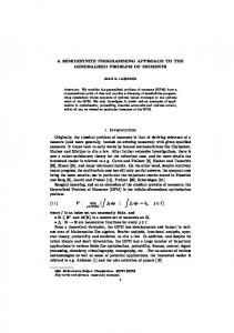
unimodal distributions, with the same moments6 up to order k, where k = 2, . . . , 10. Figure 1 plots the corresponding upper bounds Ak (a), Sk (a), SUk (a) and the normal sdf N (a) as functions of a ≥ 0; the three plots correspond to k = 2, 4 and respectively 10 moments. While all bounds perform well in the tails (beyond 3-4 std), the bound for symmetric and unimodal distributions exhibits a good performance also around the mean.

1

1

k=2

0.9

1

k=4

0.9

0.8

0.8

0.8

0.7

0.7

0.7

0.6

0.6

0.6

0.5

0.5

0.5

0.4

0.4

0.4

0.3

0.3

0.3

0.2

0.2

0.2

0.1

0

0.1

0

0.5

1.5

1

2.5

2

3.5

3

4.5

4

0

5

k=10

0.9

0.1

0

0.5

1.5

1

2.5

2

a

3.5

3

4.5

4

0

5

0

0.5

1.5

1

2.5

2

a

3.5

3

4.5

4

5

a

Figure 1: From left to right: bounds given k = 2, 4, 10 moments respectively. Each plot compares Ak (a), Sk (a), SUk (a) and N (a) for a ∈ [0, 5].

1

1

Ak(a)

0.9

1

Sk (a)

0.9

0.8

0.8

0.8

0.7

0.7

0.7

0.6

0.6

0.6

0.5

0.5

0.5

0.4

0.4

0.4

0.3

0.3

0.3

0.2

0.2

0.2

0.1

0

0.1

0

0.5

1

1.5

2

2.5

a

3

3.5

4

4.5

5

0

SUk(a)

0.9

0.1

0

0.5

1

1.5

2

2.5

3

3.5

4

4.5

5

0

0

0.5

1

1.5

2

a

2.5

3

3.5

4

4.5

5

a

Figure 2:

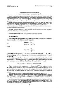
From left to right: Ak (a), Sk (a) and SUk (a), a ∈ [0, 5]. Each plot compares sharp bounds given k = 2, 4, 10 moments vs. the normal sdf.

In Table 1 we compare the improvement of the bound for symmetric unimodal distributions over the bound for arbitrary distributions, relative to the normal sdf benchmark, calculated as ∆k (a) = (Ak (a) − SUk (a))/(Ak (a) − N (a)). Remarkably, ∆k (a) is consistently (i.e. for all a and k) above 75%. It is higher around the mean, for any number of moments, and it is also higher in the tails for moments of higher order. It is interesting to understand how much the various bounds improve as higher order moments are given. Each plot in Figure 2 compares the bounds given 2, 4 and 10 moments (against the normal sdf benchmark) for a category of distributions: arbitrary, symmetric, respectively unimodal and symmetric. The value of adding higher order moment information appears to be higher under less distributional assumptions. In fact, for unimodal and symmetric distributions, the mean-variance bound (k = 2) is already fairly strong. This also shows that approximating a unimodal and symmetric distribution by a normal with the same mean and variance yields a reasonably good approximation. Another interesting observation is that fourth moment information has a most significant impact in the tails (beyond 2 − 2.5 standard deviations), but less so around the mean. This can also be observed from Table 2, which illustrates the relative improvement in the bound for symmetric unimodal distributions from using higher order moments ∆su k (a) = (SUk (a) − SUk+2 (a))/(SUk (a) − N (a)). The relative 6 The

first ten moments of the standard normal distribution are M = (0, 1, 0, 3, 0, 15, 0, 105, 0, 945).


18

a 0 0.2 0.4 0.6 0.8 1.0 1.2 1.4 1.6 1.8 2.0 2.2 2.4 2.6 2.8 3.0 3.2 3.4 3.6 3.8 4.0 4.2 4.4 4.6 4.8 5.0

∆2 (a) 100 96.01 92.29 88.61 85.62 84.59 86.70 87.32 85.85 83.64 81.49 79.66 78.24 77.29 76.74 76.29 76.22 76.17 76.33 76.35 76.36 76.49 76.58 76.72 76.92 76.88

∆4 (a) 100 93.92 89.33 86.32 84.82 84.59 85.95 84.59 80.26 79.88 83.03 85.28 86.20 86.26 85.56 84.44 84.27 83.92 84.35 84.04 84.42 84.38 84.91 84.09 86.49 84.38

∆6 (a) 100 96.27 93.13 91.16 91.82 90.91 87.01 82.90 79.80 79.75 81.48 81.35 79.17 80.60 82.71 82.42 82.54 82.22 83.87 82.61 82.35 84.62 80.00 85.71 83.33 75.00

∆8 (a) 100 95.46 92.33 90.95 91.79 90.20 86.39 87.19 89.04 88.81 86.79 83.02 79.03 78.92 78.30 75.81 80.56 81.82 84.62 87.50 83.33 75.00 100 100 100 100

∆10 (a) 100 96.69 94.24 93.77 93.27 88.98 85.99 87.16 88.37 86.58 85.24 86.15 85.10 82.56 79.25 75.00 78.13 76.47 75.00 75.00 76.67 100 100 100 100 100

Table 1: Percentage improvement of the bound for symmetric unimodal distributions over the bound for arbitrary distributions (relative to the normal), given k =2,4,6,8, and 10 moments.

a 0.2 0.4 0.6 0.8 1.0 1.2 1.4 1.6 1.8 2.0 2.2 2.4 2.6 2.8 3.0 3.2 3.4 3.6 3.8 4.0 4.2 4.4 4.6 4.8 5.0

∆su 2 (a) 0 0 0 0 0 0 0 0 0.0469 0.3089 0.5732 0.7156 78.62 84.05 85.04 86.67 87.83 89.35 90.20 91.37 92.06 93.04 93.33 94.79 94.38

∆su 4 (a) 0 41.20 44.61 50.86 62.41 58.94 29.34 2.76 0 0 0 0 0 43.90 54.29 60.71 65.22 72.22 73.33 75.00 80.00 75.00 85.71 80.00 80.00

∆su 6 (a) 0 0 0 0 0 0 13.72 44.16 60.66 57.08 37.14 10.99 0 0 6.25 36.36 50.00 60.00 75.00 66.67 50.00 100 100 100 100

∆su 8 (a) 0 29.92 33.94 43.80 33.02 0.46 0 0 0.83 0 14.77 38.27 23.08 4.35 0 0 0 0 0 0 100 NaN NaN NaN NaN

Table 2: Percentage improvement in the bound for symmetric unimodal distributions relative to the normal sdf due to higher moment information. (NaN stand for division by zero.)


19

improvement from using higher order moments appears to be much stronger in the tails than around the mean. Nevertheless, no monotonicity relationship can be observed. The numerical experiments have been conducted in MATLAB5.3 under WindowsXP, using the SOS Toolbox [27]- an optimization package over semi-algebraic sets, based on the SeDuMi [39] solver for semidefinite programming. 8. Conclusions. In this paper we showed how optimal moment bounds over convex classes of distributions generated by one-parameter families can be efficiently computed using semidefinite programming. Polar representations and conic duality provide a general and tractable framework for solving Problem (P) for convex classes of distributions, satisfying special properties such as symmetry, unimodality, convexity and smoothness. We also extended these results to obtain approximate SDP solutions for multi-parameter classes and multivariate distributions. Finally, we applied these results to obtain generalizations of Chebyshev’s inequality given higher order moments via SDP. Numerical computation shows that accounting for structural properties such as symmetry and unimodality can improve the quality of the moment bounds by at least 75%. Appendix A. Proof of Proposition 3.1. The first part of the proposition is a known result. We provide a proof for completeness: R Clearly cx(T ) ⊆ mix(T ). To prove mix(T ) ⊆ cx(T ), let µ = τ dν(τ ) ∈ mix(T ). The set of measures with finite support is weakly dense in M+ (T ) (a separable metric space7 ), so there exists R νn → ν such that R νn has support on (at most) n points. Let µn = τ dνn (τ ) ∈ cx(T ). For any bounded continuous h, in τ ∈ T (in the inherited weak topology), implying R R ¡R hdτ¢ is bounded R ¡R and¢ continuous R hdµn = hdτ dνn → hdτ dν = hdµ, so µ ∈ cx(T ). This concludes the proof of the first part. The second part of Proposition 3.1 is not new in the compact case. It follows from the following result (Phelps [29, Proposition 1.2] ): Proposition A.1 Suppose that X is a compact subset of a locally convex8 topological space. Then cx(X) = mix(X). Since the space of probability measures can be appropriately metrized, weak compactness is sufficient. By Prohorov’s Theorem (see Billingsley [5]), a sufficient condition for weak compactness is that T be weakly closed and uniformly tight, i.e. for any ² > 0 there exists a compact K² with τ (K² ) > 1 − ² for every τ ∈ T . Uniform tightness is satisfied if Ω is compact. For non-compact intervals Ω ⊆ R, the following proof has been suggested by Edgar [11]. Consider for ¯ example Ω = [0, ∞) (the other cases work similarly), which is not compact, but can be compactified in R ¯ by adding the point {∞}. This yields Ω = [0, ∞], which is homeomorphic to [0, 1]. The set of probability ¯ : M+ (Ω) = measures on Ω can be identified with the following subset of probability measures on Ω + ¯ {µ ∈ M (Ω) | µ({∞}) = 0}. ¯ Let S denote the closure of T in M+ (Ω). Since T is closed in M+ (Ω), it follows that T = {µ ∈ S | µ({∞}) = 0}. By Proposition A.1 we have cx∗ (S) = mix(S), where the star refers to ¯ closure in M+ (Ω). We want to show that cx(T ) ⊆ mix(T ), where the closure is in M+ (Ω). Let µ0 ∈ cx(T ). Then µ0 ∈ cx∗ (S) and µ0 ({∞}) = 0. Let ν0 ∈ M+ (S) be a mixing measure for µ0 . It remains to show that ν0 is concentrated on T . For this we rely on the following result (Phelps [29, Chapter 12, p. 100] ): Proposition A.2 If X is a compact convexR subset of a locally convex space and if ν is a probability measure on X with resultant x, then f (x) = f dν for each affine function f of first Baire class. Affine functions of first Baire class are those affine functions that are the pointwise limit of a sequence of continuous (not necessarily affine) functions on X. The map µ → µ({∞}) is affine and of first Baire 7 It

is possible to metrize the space of probability measures as a separable complete metric space such that convergence in the metric is equivalent to weak convergence (see Parthasarathy [28, Theorem 6.2 Ch. II]) 8 A space is locally convex if it admits a convex base. Any metric space is locally convex.


20

class (although not continuous). To see this, R use continuous increasing functions fn (x) that are zero for x < n, and one for x > n + 1. Then each fn dµ is continuous, and µ({∞}) is the limit of that sequence. R Therefore, by Proposition A.2, 0 = µ0 ({∞}) = S µ({∞})dν0 (µ). This integral of a non-negative function is zero, so the set {µ ∈ S | µ({∞}) = 0} = T has ν0 -measure 1. This shows that ν0 is supported on T , so µ0 ∈ mix(T ), as claimed. The above argument easily extends for closed sets Ω ⊆ Rm , using the one-point compactification of R (i.e. add one extra point ∞, with neighborhoods consisting of the complements of the compact sets of Rm ). This result becomes relevant in Section 6, when we deal with multivariate extensions. m

Appendix B. Proofs of Lemmas 5.1 and 5.2. Proof of Lemma 5.1. We only prove part (a); the second part is analogous. Any measure in dx S = cx(Tm,a ) admits a continuous piecewise linear decreasing and convex density. Conversely, any continuous piecewise linear decreasing and convex density function on [m, m + a], can be written as Pl p(x) = s0 + i=1 si (bi −x)+ , with si ≥ 0 and m ≤ bl ≤ · · · ≤ b1 ≤ m+a, where the left-slopes at breakpoints Pk Pl bk equal − i=1 si . Denote ti = bi − m and wi = si t2i /2, so p(x) = s0 + i=1 wi (2/t2i )(m + ti − x)+ . Since p(x) is a density, the weights sum up to 1. Hence the measure with density p(x) is a convex combination of triangulars and a rectangular (with weight s0 ), so it belongs in S. Hence S is the set of continuous probability measures that admit piecewise linear decreasing and convex densities. dx ix ix ¯ hence P¯m,a , so µ = αµ0 + (1 − α)δm , = S¯ as desired. Let µ ∈ P¯m,a We now show that S ⊆ P¯m,a ⊆ S, where µ0 is a continuous measure that admits an increasing convex density π0 . There exists an increasing sequence of non-negative piecewise linearR decreasing concave measurable functions πn converging R pointwise to π . By monotone convergence, π (x)dx → π (x)dx for any measurable set A. Let 0 n 0 A A R πn (x) = c1n ≤ 1, so cn → 1 and cn πn is the density function of a measure in S. Therefore the sequence R + of measures µn = αcn πn (x)dx + (1 − α)γm, 1 ∈ S converges weakly to µ0 . n

dx dx ∪ {δm }), where the Dirac at m is added to = mix(Tm,a Finally, by Proposition 3.1, we have P¯m,a insure closure of the generating set. Without it, we obtain the corresponding set of continuous measures dx dx Pm,a = mix(Tm,a ). ¤

Proof of Lemma 5.2. We only prove the first part, the second part is analogous. The proof follows dv ) admits a continuous piecewise linear the same lines as the previous lemma. Any measure in S = cx(Tm,a decreasing and concave density. Any continuous piecewise linear decreasing and concave density function Pl v(x) ≥ 0 on [m, m + a] can be written as v(x) = M − i=0 wi (x − m − ti )+ , where wi ≥ 0, 0 ≤ ti ≤ a and M = v(m + a) is the maximal value of v. It follows that

v(x) =

l X i=0

+

wi (a − ti − (x − m − ti ) ) =

l X

wi min(a − ti , a + m − x) ,

i=0

a2 −t2

which is a convex combination of right m-trapezoidal densities with weights ρi = wi 2 i ≥ 0. Since v is a density, the weights must sum to 1. This shows that S is exactly the set of distributions that admit dv dv ¯ Closure of Pm,a a piecewise linear decreasing and concave density. We now show that S ⊆ Pm,a ⊆ S. implies the desired equality. dv Let π0 be an increasing convex density for µ ∈ Pm,a . Let πn be an increasing sequence of nonnegative piecewise linear increasing convex measurable functions converging R R R pointwise to π0 . By monotone convergence, A πn (x)dx → A π0 (x)dx for any measurable set A. Let πn (x) = c1n ≤ 1, so cn → 1 and R R cn πn is the density function of a measureRin S. So cn A πn (x)dx → A π0 (x)dx for any measurable set A, and the sequence of measures µn = cn πn (x)dx ∈ S converges weakly to µ. ¤

Appendix C. Proof of Proposition 7.1. The result for arbitrary distributions is from Bertsimas and Popescu [4]. In order to simplify notation, in the following we assume that the mean M1 = 0, and hence all odd order moments are also null.


21

Symmetric random variables. According to the formulation (9) in Section 4.1, the dual of this problem can be written as: min y 0 M y

n X

s.t.

yi ((−t)2i + t2i ) ≥ 1(t≤−a) + 1(t≥a) ,

∀ t ≥ 0.

(19)

i=0

We must distinguish two cases: Case 1: a ≤ 0. By the change of variables t2 = z, we can rewrite the dual as follows: min y

s.t.

y0 M n X i=0 n X

1 2

,

for z ≥ 0

yi z i ≥ 1

,

for z ≤ a2 .

yi z i ≥

i=0

The corresponding SDP formulation is a simple application of Proposition 2 (see the explicit formulation in Bertsimas and Popescu [4]). Suppose now that n = 1, and σ 2 = M2 . The optimal Chebyshev bound for symmetric distributions is the solution of the following program: min y0 + y1 σ 2 y

s.t.

y0 + y1 z ≥ 21 y0 + y1 z ≥ 1

, ,

for z ≥ 0 for z ≤ a2 ,

The constraints imply that y0 ≥ 1 and y1 ≥ 0. It follows that the optimal bound is 1. Case 2: a > 0. By the same change of variables t2 = z, the dual can be written as: min y

s.t.

y0 M n X i=0 n X

yi z i ≥ 0

,

for z ≥ 0

1 2

,

for z ≥ a2 .

yi z i ≥

i=0

The corresponding SDP formulation is a simple application of Proposition 2 as explicitly stated in Bertsimas and Popescu [4]. Suppose now that n = 1, and σ 2 = M2 . The optimal Chebyshev bound for symmetric distributions is the solution of the following program: min y0 + y1 σ 2 y

s.t.

y0 + y1 z ≥ 0 y0 + y1 z ≥ 21

, ,

for z ≥ 0 for z ≥ a2 ,

The first constraint set is equivalent to y0 , y1 ≥ 0. In this case, the second constraint set is equivalent to y0 + y1 a2 ≥ 12 . So the problem can be reformulated as  1  µ ¶  , if σ 2 ≥ a2 1 σ2 1 2 2 2 min + y (σ − a ) = = min 1, . 2 1  2 a2 y1 ≤ 12 a2 2 2 2  σ , if σ < a 2a2 This concludes the proof of this part. Unimodal and symmetric random variables. problem can be written as:

According to formulation (12) in Section 4.4, the

min y 0 M y

s.t.

Z t n X 2yi 2i+1 t ≥ 1(x≥a) dx , 2i + 1 −t i=0

∀ t ≥ 0.

(20)


22 We consider two separate cases:

Case 1: a ≤ 0 . The equivalent dual formulation is min y 0 M y

½ n X 2yi 2i+1 2t t ≥ t−a 2i + 1 i=0

s.t.

, ,

∀ 0 ≤ t ≤ −a ∀ t ≥ −a.

(21)

The degree of the first constraint set can be reduced after simplification by 2t and the change of variable z = t2 , to n X yi z i ≥ 1 , ∀ 0 ≤ z ≤ a2 . 2i + 1 i=0 The corresponding SDP formulation is a direct consequence of Proposition 2 (see Bertsimas and Popescu [4] for the explicit formulation). For n = 1, and σ 2 = M2 , the desired bound is the solution to the following program: min y0 + y1 σ 2 y y1 s.t. y0 + z ≥ 1 3 y1 t−a y0 t + t3 ≥ 3 2

,

∀ 0 ≤ z ≤ a2

,

∀ t ≥ −a

(22)

The second constraint implies that y1 ≥ 0, whereas the first implies y0 ≥ 1. The optimum is achieved when equality holds in both, and the bound equals 1. Case 2: a > 0 . The equivalent dual formulation is: min y 0 M y

s.t.

½ n X 2yi 2i+1 0 , t ≥ t − a , 2i + 1 i=0

∀t≥0 . ∀t≥0

(23)

We degree of the first constraint can be reduced after dividing by 2t, and by the change of variable z = t2 , n X yi obtaining: z i ≥ 0 , ∀ z ≥ 0. The corresponding SDP formulation is a direct consequence of 2i + 1 i=0 Proposition 2. In particular, for n = 1 and σ 2 = M2 , we have the following program: min y1 σ 2 + y0 y y1 s.t. z + y0 ≥ 0 3 µ ¶ y1 3 1 a t + y0 − t+ ≥0 3 2 2

,

∀z ≥0

,

∀t≥0

(24)

The first condition set implies y0 ≥ 0. The second condition implies y1 ≥ 0, in which case the first constraint set is always satisfied. For y1 = 0, or y0 ≥ 21 , the bound cannot exceed 12 , obtained for y0 = 21 , y1 = 0. Suppose now that y1 > 0 and 0 ≤ y0 < 21 . Denote h(t) = y31 t3 + (y0 − 21 )t + a2 . Notice that the inflexion p point is at 0 and h(0) = a/2 ≥ 0, whereas h(a) ≥ 0. The local optima are t± = ± (1/2 − y0 )/y1 . Therefore, we can have h(t) ≥ 0 for all t ≥ a if and only if h(t+ ) ≥ 0, or else t+ ≤ a. The latter case leads 3 0) to a contradiction. The condition h(t+ ) ≥ 0 is equivalent to y1 ≥ 92 (1−2y . The minimum is achieved a2 µ ¶ 2 1 2 σ , . This concludes the proof. ¤ for y0 = 0 or y0 = 12 , and the value of the bound is min 2 9 a2 Acknowledgments. The author is particularly grateful to Gerald A. Edgar for help with the proof of Proposition 3.1. Thanks go to Frederic Bonnans, Marco Scarsini, Alexander Shapiro and Dan Timotion for pointers to the literature, to Pablo Parrilo for the opportunity to use the SOS Toolbox, and to the anonymous referees for suggestions that improved the quality of the paper.


23

References [1] N. I. Akhiezer and M. Krein, Some questions in the theory of moments, Translations of Math. Monographs, vol. 2, Amer. Math. Soc., Prov, R.I., 1962. [2] S. Bell, Approximating the normal distribution with the triangular, Tech. Report 494, Sandia Corporation Report, 1962. [3] D. Bertsimas and I. Popescu, On the relation between option and stock prices: An optimization approach, Operations Research 50 (2002), no. 2, 358–374. [4] , Optimal inequalities in probability theory: A convex optimization approach, SIAM J. Optim. (2004), forthcoming. [5] P. Billingsley, Weak convergence of measures: Applications in probability, SIAM, CBMS-NSF Regional Conference Series in Applied Mathematics, Philadelphia, PA, 1971. [6] N.P. Buslenko, D.I. Golenko, Yu.A. Shreider, I.M. Sobol, and V.G. Sragovich, The Monte Carlo Method, Oxford: Pergamon, 1966. [7] P. Chebyshev, Sur les valeurs limites des intégrales, Jour. Math. Pur. Appl. 19 (1874), no. 2, 157–160. [8] S. Dharmadhikari and K. Joag-Dev, Unimodality, convexity and applications, Probability and Mathematical Statistics, Academic Press, San Diego, CA, 1988. [9] R.M. Dudley, Real analysis and probability, Chapman and Hall Mathematics Series, New York, 1989. [10] R.J. Duffin, Infinite programs, Linear inequalities and related systems (H. W. Kuhn and A. W. Tucker, eds.), Princeton University Press, Princeton, NJ, 1956, pp. 157–170. [11] G.A. Edgar, personal communication, March 2004. [12] G. Gallego, A minmax distribution free procedure for the (q,r) inventory model, Oper. Res. Letters 11 (1992), 55–60. [13] L. El Ghaoui, M. Oks, and F. Oustry, Worst-case value-at-risk and robust portfolio optimization: A conic programming approach, Operations Research 51 (2003), no. 4, 543–556. [14] B. Grundy, Option prices and the underlying asset’s return distribution, Journal of Finance 46 (1991), no. 3, 1045–1070. [15] K. Isii, On the sharpness of Chebyshev-type inequalities, Ann. Inst. Stat. Math. 14 (1963), 185–197. [16] S. Karlin and W.J. Studden, Tchebycheff systems: with applications in analysis and statistics, Pure and Applied Mathematics, A Series of Texts and Monographs, Interscience Publishers, John Wiley and Sons, 1966. [17] A.F. Karr, Extreme points of certain sets of probability measures with applications, Math. Oper. Res. 8 (1983), no. 1, 74–85. [18] A.Y. Khintchine, On unimodal distributions, Izv. Naucho-Isled. Inst. Mat. Mech. Tomsk. Gos. Univ. 2 (1938), 1–7. [19] G. Lanckriet, L. El Ghaoui, C. Bhattacharya, and M. Jordan, Minimax probability machine, working paper, University of California, Bekeley, 2001. [20] H.J. Landau, Classical background on the moment problem, Moments in Mathematics (Providence, RI) (ed. H.J. Landau, ed.), Proc. Sympos. Appl. Math., Series III, no. 37, American Mathematical Society, 1987, pp. 1–15. [21] M. LiCalzi, Upper and lower bounds for expected utility, Economic Theory 16 (2000), 489–502. [22] A. Lo, Semiparametric upper bounds for option prices and expected payoffs, Journal of Financial Economics 19 (1987), 373–388. [23] C.L. Mallows, Generatizations of Tchebysheff ’s inequalities, J. Roy. Stat. Soc. 18 (1956), no. 2, 139–168. [24] A. Markov, On certain applications of algebraic continued fractions, Ph.D. thesis, St. Petersburg, 1884, in Russian. [25] H.P. Mulholland and C.A. Rogers, Representation theorems for distribution functions, Proc. London Math. Soc. 3 (1958), no. 8, 177–223. [26] Y. Nesterov, Structure of non-negative polynomial and optimization problems, Preprint DP 9749, Louvan-laNeuve, Belgium, 1997. [27] P. Parrilo, Sos toolbox (algorithm for optimization over semi-algebraic sets), ETH, Zurich, Switzerland, http://www.cds.caltech.edu/sostools/, 2002. [28] K.R. Parthasarathy, Probability measures on metric spaces, Academic Press, New York etc., 1967. [29] R.R. Phelps, Lectures on Choquet’s Theorem, van Nostrand Mathematical Studies, New York etc., 1966. [30] M. Putinar, Positive polynomials on compact semi-algebraic sets, Indiana University Mathematics Journal 42 (1993), no. 3, 969–984. [31] R.T. Rockafellar, Convex analysis, Princeton University Press, Princeton, NJ, 1970. [32] W.W. Rogosinsky, Moments of non-negative mass, Proc. Roy. Soc. London. Ser. A. 245 (1958), 1–27. [33] H. Scarf, A min-max solution of an inventory problem, Studies in the mathematical theory of inventory and production (Stanford University Press, Stanford, CA), K.J. Arrow, S. Karlin and H. Scarf, eds., 1958, pp. 201–209.

24


[34] A. Shapiro, On duality theory of conic linear problems, Semi-infinite programming: recent advances (M.A. Goberna and M.A. Lopez, eds.), Kluwer Academic Publishers, 2001, pp. 135–165. [35] J.A. Shohat and J.D. Tamarkin, The problem of moments, Mathematical Surveys, American Mathematical Society, New York, 1943. [36] J. Smith, Generalized Chebyshev inequalities: Theory and applications in decision analysis, Operations Research 43 (1995), no. 5, 807–825. [37] J.B. Soll and J. Klayman, Soverconfidence in interval estimates, Journal of Experimental Psychology: Learning, Memory, and Cognition 30 (2004), 299–314. [38] T.J. Stieltjes, Recherches sur les fractions continues, Annales de la Faculté de Sciences de Toulouse 9 (1895), no. 1, 5–47. [39] J. Sturm, SeDuMi (semidefinite programming algorithm), version 1.05, Department of Econometrics, Tilburg University, The Netherlands, http://fewcal.kub.nl/sturm/software/sedumi.html, 1998. [40] Y.L. Tong, Probability inequalities in multivariate distributions, New York, Academic Press, 1980. [41] J.V. Uspensky, Introduction to mathematical probability, McGraw-Hill, New York, 1937. [42] H. Weizs¨ acker and G. Winkler, Integral representation in the set of solutions of a generalized moment problem, Math. Ann. 246 (1979), 23–32. [43] Y. Willassen, Best upper and lower Tchebycheff bounds on expected utility, Review of Economic Studies 57 (1990), 513–520. [44] G. Winkler, On the integral representation in convex noncompact sets of tight measures, Math. Z. 158 (1978), 71–77. [45] H. Wolkowicz, R. Saigal, and L. Vandenberghe editors, Handbook of semidefinite programming, theory, algorithms, and applications, Kluwer Academic Publishers, 2000. [46] Y. Yamada and J. Primbs, Value-at-risk (VaR) estimation for dynamic hedging, International Journal of Theoretical and Applied Finance 5 (2002), no. 4, 333–354.