American Journal of Operations Research, 2014, 4, 293-300 Published Online September 2014 in SciRes. http://www.scirp.org/journal/ajor http://dx.doi.org/10.4236/ajor.2014.45028
Safe Bounds in Semidefinite Programming by Using Interval Arithmetic Orkia Derkaoui1, Ahmed Lehireche2 1
Computer Science Department, University Dr Moulay Tahar of Saida, Saida, Algeria Computer Science Department, University Djillali Liabes of SidiBel Abbes, SidiBel Abbes, Algeria Email:
[email protected],
[email protected]
2
Received 29 April 2014; revised 10 June 2014; accepted 6 August 2014 Copyright © 2014 by authors and Scientific Research Publishing Inc. This work is licensed under the Creative Commons Attribution International License (CC BY). http://creativecommons.org/licenses/by/4.0/
Abstract Efficient solvers for optimization problems are based on linear and semidefinite relaxations that use floating point arithmetic. However, due to the rounding errors, relaxation thus may overestimate, or worst, underestimate the very global optima. The purpose of this article is to introduce an efficient and safe procedure to rigorously bound the global optima of semidefinite program. This work shows how, using interval arithmetic, rigorous error bounds for the optimal value can be computed by carefully post processing the output of a semidefinite programming solver. A lower bound is computed on a semidefinite relaxation of the constraint system and the objective function. Numerical results are presented using the SDPA (SemiDefinite Programming Algorithm), solver to compute the solution of semidefinite programs. This rigorous bound is injected in a branch and bound algorithm to solve the optimisation problem.
Keywords Semidefinite Programming, Interval Arithmetic, Rigorous Error, Bounds, SDPA Solver, Branch and Bound Algorithm
1. Introduction We consider the standard primal semidefinite program in block diagonal form:
p* = min c T x s.t.= X
m
∑Fi xi − F0 , i =1
where c =
( c1 ,, cm )
T
∈
m
is the cost= vector, x
( x1 ,, xm )
X 0, T
(1)
∈ m is the variables vector and the matrices
How to cite this paper: Derkaoui, O. and Lehireche, A. (2014) Safe Bounds in Semidefinite Programming by Using Interval Arithmetic. American Journal of Operations Research, 4, 293-300. http://dx.doi.org/10.4236/ajor.2014.45028
O. Derkaoui, A. Lehireche
Fi ∈ S for i = 0, , m are matrices in S n . Recall that S n denotes vector space of real symmetric n × n matrices and X 0 means that X ∈ S+n , the cone of positive semidefinite matrices in S n . p* is the optimal value of the primal objective function. The standard inner product on S n is:
(
)
A= ⋅ B tr ( AB = ) tr AT B , ( where tr = ( A) trace ( A) ) , with A and B ∈ S n .
The dual semidefinite program of (1) is: = d * max = d * max F0 ⋅ Y s.t.
F = c= 1, , m ) , i ⋅Y i , (i
Y 0,
(2)
with Y ∈ S+n and d * is the optimal value of the dual objective function. ( x, X ) is a feasible (minimum) and (or optimal) solution of the primal semidefinite problem (1) and Y is a feasible (maximum) and (or optimal) solution of the dual semidefinite problem (2). The duality theory for semidefinite programming is similar to its linear programming counterpart, but more subtle (see for example [1]-[3]). The programs satisfy the weak duality condition: d * ≤ p* . Interior point methods are a certain class of algorithms to solve most of semidefinite programs [4]-[7]. However, due to the use of floating point arithmetic, these algorithms may produce erroneous results. That is to say, when run on a computer, the result of these algorithms could be an overestimation or, worst, an underestimation of the very global optima. The purpose of this article is to show how rigorous error bounds for the optimal value can be computed by carefully post processing the output of a semidefinite programming solver. We use interval computation to rigorously bound the global optima. Thus the use of outward rounding allows a safe bounding of the global optima. There exist many solvers of semidefinite programs which provide tight bounds as pointed out in Roupin et al. (see, e.g., [8]), however they are unsafe. That is why we propose here to embed safe semidefinite relaxations in an interval framework. Before going into details, let us show, in a small example, a flaw or lack of rigor on the computation of the optimal value of the objective function [9]. Consider the following optimization problem: min x s.t.
y − x2 ≥ 0 y − x 2 ( x − 2 ) + 10−5 ≤ 0
(3)
x, y ∈ [ −10, +10]
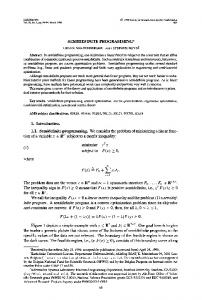
As shown in Figure 1, the solution of problem (3) lies in the neighbourhood of point x ≈ 3, y ≈ 9 . This point is the unique intersection of curve y = x 2 and curve y= x 2 ( x − 2 ) − 10−5 . However, at point = x 0,= y 0, two curves are only separated by small distance of 10−5. Using Baron (6.0 and 7.2) [9], a solver based on the techniques of relaxations, in particular linear and convex relaxations, quickly it finds 0 as global minimum even if the precision is enforced up to 10−12 . Such a flaw is particularly annoying: as pointed out in [10], there are many situations, like safety verification problem or chemistry, where the knowledge of the very global optima is critical.
Figure 1. Geometrical representation of Problem (3).
294
O. Derkaoui, A. Lehireche
The rest of this paper is organized as follows. The next section contains notations. In Section 3 an overview of the use of a procedure to compute a rigorous semidefinite bound is considered, and Section 4 contains numerical results. Finally, in Section 5, we provide some concluding remarks.
2. Notations, Interval Arithmetic We require only some elementary facts about interval arithmetic, which are described here. There are a number of textbooks on interval arithmetic and selfvalidating methods that we highly recommend to readers. These include Alefeld and Herzberger [11], Moore [12], and Neumaier [13]. x = [ x , x ] = x ∈ m∕x ≤ x ≤ x is called an interval vector with lower bound x and upper bound x . x , y denote indifferently intervals and vectors of intervals, also called boxes. The width w ( x ) of the interval x is the quantity x − x . The interval evaluation of a real-valued function f ( x ) is an interval f . f * and f * , respectively, denote lower and upper bounds of f * , the optimal value of the objective function f . For interval vector A we define A+ = max {0, A} and A− = max {0, A} . All interval operations can be easily executed by working appropriately with the lower and upper bounds of the intervals.
{
}
3. Rigorous Lower Bound Semidefinite programs are typically used in branch-and-bound algorithms, to find lower bounds on the objective that allow one to decide whether a given node in the branch tree can be fathomed. For reliable results, it is therefore imperative that the computed lower bound is rigorously valid. However, the output of semidefinite programming routine is the result of an approximate calculation and hence is itself approximate. Obtaining rigorous error bounds for the solution of semidefinite problems is a difficult task [14]. Fortunately, it is possible to post process the approximate result to obtain rigorous bounds for the objective with reasonable effort, using directed rounding and interval arithmetic. The most famous implementation of this approach with linear relaxations are documented by many applications and a number of survey papers (for example Lebbah et al. [9]). Recently, Neumaierand Shcherbina [15] proposed in the context of linear programming a safe procedure mathematically proven witch computes bound and guarantees its rigor. We introduce in this paper an extension of this procedure on semidefinite programming. As pointed out in Neumaier and Shcherbina [15], using directed rounding and interval arithmetic, cheap post processing of the linear programs arising in branch and bound framework can guarantee that no solution is lost. In mixed integer programming, linear programs are typically used to find lower bounds on the objective that allow one to decide whether a given node in the branch tree can be fathomed. For reliable results, it is therefore imperative that the computed lower bound is rigorously valid. However, the output of a linear programming routine is the result of an approximate calculation and hence is itself approximate [16]. Obtaining rigorous error bounds for the solution of linear programming problems is a difficult task (cl. KRAWCZYK [17], JANSSON [18], JANSSON & RUMP [19]). Fortunately, it is possible to post process result to obtain rigorous bounds for the objective with reasonable effort, provided that reasonable bounds on all variables are available. Such bounds are frequently computed anyway in a preprocessing phase using a limited form of constraint propagation, and if the latter is done with sufficient care (using directed rounding to ensure the mathematical validity of each step of the process) [20] [21], these bounds on the variables are rigorously valid. We begin by looking at the simpler case where the linear program is given in the standard form.
min c T x s.t. = Ax b, x ≥ 0.
(4)
Its dual is max bT y s.t.
AT y ≤ c, y ≥ 0.
Thus a rigorous lower bound µ for c T x is obtained as follows. roundup :
295
(5)
O. Derkaoui, A. Lehireche
µ = +T b; = r AT y − c;
(6)
roundup :
(
)
r =max −r , AT +c ;
µ= −T b − µ + r T max ( − x, x ) ; µ = −µ; Of course, there are a variety of other ways of doing the estimates, e.g., using suitable case distinctions, and a high quality implementation would have to test which one is most efficient. We use the extension of this result to semidefinite program. We solve the semidefinite program (8) below and its dual (9) with the SDPA [4], a software package for solving semidefinite programs. It is based on a Mehrotratype predictor-corrector infeasible primal-dual interior-point method [5] [6]. We post process the output of the solver to obtaining rigorous error bounds for the optimal value. To simplify the formulas, we use: F1 ⋅ X F ⋅ X F(X ) = 2 Fm ⋅ X
(7)
So the primal semidefinite program (1) is written: min c T x
(8)
s.t. F ( x ) − F0 = X , X 0.
And the dual semidefinite program (2) is written: max F0 ⋅ Y
(9)
F (Y ) = c, Y 0.
s.t.
The corollary below gives a rigorous value of the approximate optimal solution of the semidefinite program. Corollary 3.1.
(
c T x ≥ F0 ⋅ Y + X ⋅ Y − r T x
)
−
(10)
With x ∈ x = [ x, x ] where x and x are finite real numbers, and r ∈ r =[ r , r ] . Proof: Solving the problem with the SDPA solver, we obtain ( x, X ) an approximate solution of the primal program (8) and Y an approximate solution of the dual program (9). We obtain the corollary as follows:
( F (Y ) − c ) ,
= r F (Y ) − c, r is the residuel
so we obtain:
= c F (Y ) − r = cT
( F (Y ) − r )
= cT x
( F (Y ) − r )
= cT x
( F (Y ) )
T
T
T
x
x − rT x
We replace F(Y) with its expression (7), we obtain: = cT x
( tr ( F Y ) tr ( F Y ) tr ( F Y )tr ( F Y ) ) x − r 1
2
Knowing that tr ( A ) + tr ( B ) =tr ( A + B ) , we obtain:
296
3
m
T
x
= cT x
( tr ( F x Y ) tr ( F x Y ) tr ( F x Y )tr ( F 1 1
2 2
3 3
x Y )) − r T x
O. Derkaoui, A. Lehireche
m m
= c T x tr ( F1 x1Y + F2 x2Y + F3 x3Y + + Fm xmY ) − r T x = c T x tr ( ( F1 x1 + F2 x2 + F3 x3 + + Fm xm ) Y ) − r T x
= c T x tr
From the problem (1), we have
∑ i =1 Fi x=i m
(( ∑
m i =1
) )
Fi xi Y − r T x
F0 + X , so we obtain:
c T x = tr ( ( F0 + X ) Y ) − r T x
c T x = tr ( F0Y ) + tr ( XY ) − r T x And thus:
c T x = F0 ⋅ Y + X ⋅ Y − r T x
(11)
Extending (11) on the intervals, and assuming that rigorous two-sided bounds [ x , x ] on x are available, and the two-sided bounds [ r , r ] on r are obtained by simple interval computation. We obtain the final formula that provides a rigorous lower bound of c T x
(
c T x ≥ F0 ⋅ Y + X ⋅ Y − [ r , r ]
T
[ x , x ])
−
(12)
Inexact arithmetic, r = 0, and we have at the optimum XY = 0 (complementary slackness between X and Y from the optimality conditions). Then in (12) we obtain c T x = F0 ⋅ Y which is consistent with the duality theorem (at the optimum, the primal objective c T x is equal to the dual objective F0 ⋅ Y ). This result is used to have a lower bound of the objective function and then we assumed the completeness of the algorithm branch and bound.
4. Global Optima To solve optimization problem, the branch-and-bound procedures sequentially generate semidefinite programming relaxations. However, due to the rounding errors, relaxation thus may overestimate, or worst, underestimate the very global optima [22]. A consequence is that the global optima may be cut off. To avoid this disadvantage we can apply the algorithms for computing rigorous bounds described in the previous sections. Therefore, the computation of rigorous error bounds, which take account of all rounding errors and of small errors, is valuable in practice. Therefore the experimentation results show that by properly post processing the output of a semidefinite solver, rigorous error bounds for the optimal value can be obtained. The relaxation is solved with the SDPA which handles the standard form of the SDP problem and its dual. The quality of the error bounds depends on the quality of the computed approximations and the distances to dual and primal infeasibility. By comparing these bounds, one knows whether the computed results are good.
5. Experimentations Numerical Results In this section, we present some numerical experiments for solving rigorously semidefinite problems. The results were obtained by using the solver SDPA witchhandles the standard form of semidefinite program and its dual [4]. To test our procedure of correction, we generated linear programs automatically and particular quadratic programs, for which we know the primal objective value. We thus allow to validate our procedure in experiments with comparison. The solver SDPA solves the semidefinite relaxation of the problem considered and then we apply our procedure to the results. The motivation to consider these examples is to show the effectiveness and the realizability of our procedure. We consider the linear program:
297
O. Derkaoui, A. Lehireche
min ∑ m xi i =1 LP . . 3 − s t xi = 1, ( i = 1, , m ) .
(13)
And we consider the quadratic program:
min ∑ m xi i =1 QP 2 xi 2,= ( i 1,, m ) . s.t.=
(14)
We use the standard format of the Input Data File. In [23] the structure of the input SDP problem file is given as follows: Title and comments m—number of the primal variables xi nBLOCK—number of blocks bLOCKsTRUCT—block structure vector c F0 F1 . . . Fm SDPA handles Fi matrices blocks. This strategy minimizes the computational cost during SDP problem solving. It uses the term number of blocks noted Nblock. The SDPA stores computational results in the output file such as an approximate optimal solution, the total number of iteration, the primal objective function value, the dual objective function value and other final informations. Table 1 and Table 2 present the results of our experimentations. In these tables, Prob is the problem (13) in Table 1 and the problem (11) in Table 2, m is the number of variables, P is the approximate objective function ( p* ) of the problem (10) gives by SDPA solver, PC is the rigorous objective function ( p* ) gives by our procedure , safe is a flag that indicates whether the objective function is rigorous (+) or not (−), Ex is the exact value of objective function and Ec is the gap (Ex – PC). Below, some results are presented, obtained on some well-known benches with the branch and bound solver. Audet’s problems come from his thesis [24]. The presented results can be viewed as a further development of similar methods for linear programming. Table 3 presents the results of our experimentations of global bound. In this table, Prob is the problem to solve, m is the number of variables, n is the number of constraints, Ntot is the total of nodes, Nopt is the optimal node, Lower is the rigorous objective function of the problem gives by our procedure with SDPA solver, Upper is the upper bound, and CPU is the time in second required to solve the problem. We note that throughout the test database, our solver supervises the actual optimal solution always correctly. This rigor in resolution with the SDPA solver is crucial because it guarantees us completeness. Therefore, their integration into the branch and bound algorithms is plausible. These results show that the use of interval arithmetic computation gives rigorous bounds. We can always use filtering techniques and parallelism to optimize the quality of the solution and the CPU time. Table 1. Rigorous lower bound of problem (13). SDPA Prob
SDPA + correction
m P
safe
PC
safe
Ex
Ec
LP 10
10
3.33333339
−
3.333333333331
+
10/3
2.23e−13
LP 100
100
3.33333339
−
3.33333333330
+
100/3
2.33e−12
LP 300
300
100.000001
−
99.99999999992
+
100
0.00000000007
LP 400
400
133.333335
−
133.33333333332
+
400/3
1.33e−11
298
O. Derkaoui, A. Lehireche
Table 2. Rigorous lower bound of problem (14). SDPA Prob
SDPA + correction
m P
safe
PC
safe
Ex
Ec
QP 10
10
−14.142135464476482
−
−14.1421362557497349
+
−10 2
6.32e−7
QP 100
100
−141.42135464476488
−
−141.421362557495911
+
−100 2
6.32e−6
QP 300
300
−424.26406393429477
−
−4274.264087672501047
+
−300 2
1.89e−5
QP 400
400
−565.68541857905973
−
−565.6854502300093372
+
−400 2
2.52e−5
Table 3. Global optima Audet’s problems. Exemple
m
n
Ntot
Nopt
Lower
Upper
CPU
Audet 140 a
4
5
349
221
−4.539305707658855900e+002
−4.499999990971213e+02
2.00e+001
Audet 140 a0
5
6
349
67
−4.678171282852730400e+002
−4.649489795900000200e+002
2.56e+000
Audet 140 b
3
4
349
119
8.574005320128242600e+003
1.012664433619846e+004
5.87e+000
Audet 141
4
6
349
25
2.218693168143023500e+000
1.701631618840739e+01
3.00e−001
Audet 142
3
4
349
16
−6.654110694046532400e+003
−5.450750000000000000e+003
6.00e−002
Audet 145
9
7
349
341
−1.222050857361459700e+003
−9.688446461405747000e+002
7.00e+001
Audet 146
17
10
349
91
6.512230733117274900e+001
6.64865039370471322400e+01
8.53e+000
Audet 147
22
16
349
7
1.44012460794244500e+002
1.577915241468272100e+002
7.00e−002
Audet 149
24
10
349
34
3.869747570739851900e−003
4.332831646192127900e−001
1.58e+000
6. Conclusion and Future Works The computation of rigorous error bounds for semidefinite optimization problems can be viewed as a carefully post processing tool that uses only approximate solutions computed by a semidefinite solver. In this paper, we have introduced a safe and efficient framework to compute a rigorous solution of semidefinite relaxation of a nonlinear problem. Our numerical experiments demonstrate that, roughly speaking, rigorous lower bounds for the optimal value are computed even for semidefinite programs. The numerical results show that such rigorous error bounds can be computed even for problems of large size.
References [1]
Nemirovski, A. (2003) Lectures on Modern Convex Optimization.
[2]
Ramana, M.V., Tunçel, L. and Wolkowicz, H. (1997) Strong Dality for Semidefinite Programming. SIAM Journal on Optimization, 7, 641-662. http://dx.doi.org/10.1137/S1052623495288350
[3]
Vandenberghe, L. and Boyd, S. (1996) Semidefinite Programming. SIAM Review, 38, 49-95. http://dx.doi.org/10.1137/1038003
[4]
Fujisawa, K. and Kojima, M. (1995) SDPA (Semidefinite Programming Algorithm) Users Manual. Technical Report b-308, Tokyo Institute of Technology.
[5]
Helmberg, C., Rendl, F., Vanderbei, R. and Wolkowicz, H. (1996) An Interior-Point Method for Semidefinite Programming. SIAM Journal on Optimization, 6, 342-361. http://dx.doi.org/10.1137/0806020
[6]
Vandenberghe, L. and Boyd, S. (1995) Primal-Dual Potential Reduction Method for Problems Involving Matrix Inequalities. Mathematical Programming, Series B, 69, 205-236. http://dx.doi.org/10.1007/BF01585558
[7]
Boyd, S. and Vandenberghe, L. (2004) Convex Optimization. Cambridge University Press, Cambridge. http://dx.doi.org/10.1017/CBO9780511804441
[8]
Krislock, N., Malick, J. and Roupin, F. (2012) Nonstandard Semidefinite Bounds for Solving Exactly 0-1 Quadratic Problems. EURO XXV, Vilnius.
[9]
Lebbah, Y., Michel, C., Rueher, M., Merlet, J. and Daney, D. (2005) Efficient and Safe Global Constraints for Handling Numerical Constraint Systems. SIAM Journal on Numerical Analysis, 42, 2076-2097. http://dx.doi.org/10.1137/S0036142903436174
[10] Neumaier, A. (2003) Complete Search in Continuous Global Optimization and Constraint Satisfaction. Acta Numerica.
299
O. Derkaoui, A. Lehireche
[11] Alefeld, G. and Herzberger, J. (1983) Introduction to Interval Computations. Academic Press, New York.
[12] Moore, R.E. (1979) Methods and Applications of Interval Analysis. SIAM, Philadelphia. http://dx.doi.org/10.1137/1.9781611970906 [13] Neumaier, A. (2001) Introduction to Numerical Analysis. Cambridge University Press, Cambridge. http://dx.doi.org/10.1017/CBO9780511612916 [14] Jansson, C. (2004) Rigorous Lower and Upper Bounds in Linear Programming. SIAM Journal on Optimization (SIOPT), 14, 914-935. http://dx.doi.org/10.1137/S1052623402416839 [15] Neumaier, A. and Shcherbina, O. (2004) Safe Bounds in Linear and Mixed-Integer Programming. Mathematical Programming, 99, 283-296. [16] Davis, E. (1987) Constraint Propagation with Interval Labels. Artificial Intelligence, 32, 281-331. [17] Krawczyk, R. (1995) Fehlerabschatzung bei Linearer Optimierung. In: Nickel, K., Ed., Interval Mathematics, Lecture Notes in Computer Science, Vol. 29, Springer, Berlin, 215-222. [18] Jansson, C. (1985) Zur linearen Optimierung mit unscharfen Daten. Dissertation, Fachbereich Mathematik, Universitat Kaiserslautern, Kaiserslautern. [19] Jansson, C. and Rump, S.M. (1991) Rigorous Solution of Linear Programming Problems with Uncertain Data. Zeitschrift für Operations Research, 35, 87-111. [20] Benhamou, F. and Older, W. (1997) Applying Interval Arithmetlc to Real, Integer and Boolean Constraints. Journal of Logic Programming, 32, 1-24. [21] Berkelaar, M. (2005) Lpsolve 5.5, Free Solver, lpsolve.sourceforge.net. Technical Report, Eindhoven University of Technology, Eindhoven. [22] Kearfott, R.B. (1996) Rigorous Global Search: Continuons Problems. [23] Fujisawa, K., Fukuda, M., Kobayashi, K., Kojima, M., Nakata, K., Nakata, M. and Yamashita, M. (2008) SDPA (Semidefinite Programming Algorithm) and SDPA-GMP User’s Manual—Version 7.1.1. [24] Audet, C. (1997) Optimisation globale structurée: Propriétés, équivalences et résolution. Ph.D. Thesis, École Polythecnique de Montréal, Montréal.
300