molecular dynamics. Eric Barth, Margaret Mandziuk and Tamar Schlick ...... Ryckaert, J.P., Ciccotti, G. and Berendsen, H.J.C., J. Comput. Phys., 23(1977)327. 16.
A separating framework for increasing the timestep in molecular dynamics Eric Barth, Margaret Mandziuk and Tamar Schlick Department of Chemistry and Courant Institute of Mathematical Sciences, The Howard Hughes Medical Institute and New York University, 251 Mercer Street, New York, NY 10012, US.A.
Introduction In molecular dynamics (MD) simulations, the Newtonian equations of motion are solved numerically, and a space/time trajectory of the molecular system is obtained [1,2]. Typically, explicit integration algorithms are used: new positions and velocities for all atoms are computed in closed form through simple relations involving positions and velocities at previous steps. Standard explicit schemes are simple to formulate and fast to propagate, but they impose a severe restriction on the integration timestep size: .::\t must resolve the most rapid vibrational mode [3]. This generally limits .::\t to the femtosecond (10- 15 s) range and the trajectory length to the nanosecond (10- 9 s) range. This feasible simulation range is still very short relative to motions of significant biological interest. Implicit integration algorithms [4] are widely used to increase the timestep for multiple-timescale problems where the rapid components of the motion limit numerical stability. However, implicit integrators impart two difficulties. First, the formulation is more complex, and enhanced stability is achieved at the expense of the iterative solution of a large system of nonlinear equations at each timestep. This makes the overall method computationally expensive [5]. Second, implicit integrators can damp the rapidly varying part of the solution; this is only suitable for problems where this component is rapidly decaying, with a negligible influence on the solution as time increases, which is not the case for biomolecules (at atomic resolution). Even in implicit symplectic methods, numerical damping can be realized due to a lower kinetic energy at large timesteps [6]. Both aspects (complexity and damping) introduce problems for the physical and computational effectiveness of implicit schemes for biomolecules [7-9]. The resulting trajectories at large timesteps must be carefully assessed by comparison with small-timestep trajectories, experiment, or enhancedsampling simulations. Clearly, there are two separate goals for MD simulations at large timesteps. First, if computational time were fixed per step, then certainly a larger timestep would allow the generation of trajectories spanning longer for the same computational effort. In reality, the additional cost associated with a larger integration step can still lead to an
97 W. F. van Gunsteren et al. (eds.), Computer Simulation of Biomolecular Systems © Springer Science+Business Media Dordrecht 1997
E. Barth et al.
overall competitive method if the timestep is sufficiently large. The details are methoddependent. Second, larger-timestep methods can also be useful for the enhanced sampling of configuration space. Standard explicit schemes are generally restricted, even within the nanosecond range, to a relatively small region of the thermally accessible conformation space. Thus, larger-timestep methods, which can be viewed as cruder walks in conformation space, may reveal a larger range of molecular conformations and, possibly, paths of transitions among them. Of course, larger-timestep methods do not automatically lead to enhanced sampling. In practice, they might enhance configurational sampling at the expense of full dynamical detail. Therefore, the method used should be tailored to the target problem and assessed accordingly. To evaluate current progress in this area, it is worthwhile to trace the history ofMD simulations. Since the pioneering work of Rahman [10], MD has become an important tool in many areas of biophysics and biochemistry. In the 1970s, the dynamics of molecular liquids was treated by modeling molecules as rigid rotors in generalized coordinates [11-14]. The Cartesian coordinate representation for all degrees of freedom [15] soon followed with increasing interest in larger molecular systems. In the Cartesian representation, the number of degrees of freedom is increased, but the equations of motion become simpler, allowing the simulation of larger systems. Another advantage was not fully understood until later: In Cartesian coordinates, the Hamiltonian of the system is separable - the kinetic energy depends only on the momenta and the potential energy depends only on the coordinates. This separability makes possible the use of the second-order explicit Verlet algorithm [16]. The favorable energy preservation of Verlet has long been known and was more recently explained by its symplecticness [17]. (For a comprehensive discussion of symplectic integrators, see Ref. i8.) In the absence of direct experimental data for comparison, the Verlet family of methods has become the 'gold standard' for MD simulations. With the advent of supercomputers, dynamic simulations of biological macromolecules became possible. In the pioneering work of McCammon, Gelin and Karplus [19], the small-scale motions of the protein BPTI (bovine pancreatic trypsin inhibitor, 58 residues) were followed in the Cartesian coordinates of the heavy atoms ('" 500). The hydrogen atoms were excluded, but their etrect was incorporated implicitly via effective potentials and adjustments in the masses of the heavy atoms. Researchers quickly realized that the total feasible length of MD simulations was severely limited by the small time step required to resolve the bond vibrations. This led to the SHAKE algorithm [15] and the family of multiple-time step (MTS) methods [20,21], applied to biomolecules in the pioneering work of Grubmuller et al. [22]. By constraining the bond lengths and effectively removing the most rapidly oscillating degrees of freedom, SHAKE enables timesteps two times larger compared to unconstrained methods, at a relatively small additional cost per step. MTS methods exploit the idea that the slowly varying forces can be evaluated less often than the faster components. The contribution of the slower forces to the motion can be incorporated by a Taylor expansion of the force [20,21], interpolation [23], or extrapolation [24] techniques. 98
Separating framework for increasing the MD timestep
System sizes of modeled biomolecules have increased steadily with the progress in computer hardware and the advent of parallel machines. Significantly, the total simulation time has increased far less dramatically [3,25]. Timescales of microseconds and milliseconds are still out of reach for macromolecules, and so the search for novel methodologies of simulating the dynamics of biomolecules continues. In this chapter, we review current approaches for large-time step MD and describe the progress in our normal-mode-based technique, LIN (for Langevin/Implicit integrationjNormal modes), and a related method termed LN (LIN without the implicit-integration component). The separating framework of LIN solves the Langevin equations of motion in two steps: linearization and correction. The linearized equations of motion are solved numerically by an iterative technique, the cost of which is dominated by sparse-Hessian/vector products; the resulting 'harmonic' solution is then corrected by an implicit integration step, which requires minimization of a nonlinear function. LN includes LIN's linearization, but not correction, step and emerges as more competitive in terms of CPU time. We show here through applications to the model systems of alanine dipeptide and BPTI that LIN and LN become competitive methods in comparison with traditional Verlet-like algorithms, giving similar results and a computational gain, even for small systems (e.g., a dipeptide of 22 atoms). In the next section, we briefly summarize, for a perspective, existing approaches for increasing the timestep. A description of the basic LIN framework follows, with recent algorithmic advances to improve energetic fluctuations and reduce the computational time detailed. Computational efficiency is achieved by sparse-matrix techniques, adaptive timestep selection, and fast minimization. Simulation results for alanine dipeptide and BPTI are then presented, showing good agreement with explicit-scheme simulations at 0.5 fs timesteps with respect to energetic and geometric behavior (angular distributions, rms deviations, etc.). The range of validity of the harmonic approximation is also discussed, and the performance of LN is presented. For BPTI, we demonstrate a speedup factor of 1.4 for LIN at.::\t = 15 fs, and a factor of 4.38 for LN at .::\t = 5 fs, in comparison with explicit-Langevin integration at .::\t = 0.5 fs. Already for the dipeptide, LIN at .::\t = 30 fs gives a speedup of 1.3, and LN at .::\t = 5 fs gives a factor of 2.1. These speedups for small systems contrast typical results of MTS methods, which only become more competitive as the relative number of long-range (soft) forces increases. LN, in particular, is simple to implement in general packages and should yield greater speedup for larger systems. This unexpected windfall in computational performance illustrates the value of developing novel approaches (e.g., based on normal modes) that might initially appear to be not practical for macromolecules. We conclude with a brief summary and discussion of the future applications of LIN and LN. Approaches for increasing the timestep Methods for increasing the timestep in MD can be divided into two general types: (i) constrained and reduced-variable formulations, and (ii) separating frameworks
99
E. Barth et at.
(for the system, potential, etc.). In the first category, various SHAKE-like methods are included, as well as techniques for MD in torsion space. In the second category, we consider MTS methods and reference-system methods for splitting the equations of motion, as well as novel approaches for modeling biomolecules. Constrained and reduced-variable formulations
In the various SHAKE-like methods [15,26-29], the equations of motion in Cartesian space are augmented by algebraic constraints via the formalism of Lagrange multipliers. In this way, the fastest degrees of freedom are frozen at their equilibrium values. Since the Hamiltonian remains separable, symplectic integrators which are explicit in the coordinates but implicit in the constraints can be used [30]. Recent advances in the mathematical treatment of the nonlinear systems arising in SHAKE make the method quite efficient [31]. The related reduced-variable formulations attempt to eliminate the fast degrees of freedom by modeling the system in a generalized coordinate system [32-34]. In torsion-angle dynamics [35,36], the polypeptide chain is treated as a chain of rigid bodies using a recursive rigid-body formulation [37]. Unfortunately, the reducedvariable formulations used in this class of methods destroy the separability of the Hamiltonian. Symplectic integrators like Verlet are implicit when applied to these models [18]. Therefore, in general, explicit non symplectic methods are used to propagate the dynamics in these approaches. This often leads to a drift in energy, especially at large timesteps [18]. In addition, due to constrained bond lengths and angles, the effective potential in torsion-angle dynamics is different from the original. For all these reasons, internal-variable dynamics is best suited for configurational searches (e.g., for structure refinement) at high temperatures where the interconfigurational barriers are effectively lowered. Recent results reinforce this [35,36]. Separating frameworks
MTS approaches for updating the slow and fast forces [20,22,38] form the first prototype of separating frameworks. These methods certainly provide speedup for systems with a clear division of timescales. For hydrocarbon systems such as fullerenes, the speedup is impressive (e.g., factors of 20-40) [39]. The speedup factor for biomolecules (e.g., 4) [40,41], however, is limited because such a clear division of timescales is lacking and the intramolecular coupling of modes is strong. In reference-system methods, a subset of the forces or a suitable approximation to the full force is selected for which the solution is more easily obtainable, either analytically or numerically. Examples in this category are NAPA [42] and LIN [43,44]. These methods assume that the correction to the motion - due to the complementary forces - can be obtained with a much larger timestep than that associated with the reference system. A splitting ofthe forces into linear and nonlinear parts is the premise of LIN [43,44], described in detail below. 100
Separating framework for increasing the MD timestep
Table 1 Assessment ofsome MD algorithms: Constrained dynamics (SHAKE and RAITLE), reducedvariable molecular dynamics (RVMD), multiple-timestep methods (MrS), LIN, and MOLDYN
Method
Advantages
SHAKE" RATTLEb
A doubling of feasible timestep Angles cannot be constrained (1 --+ 2 fs) is possible when bonds without affecting dynamics or are constrained convergence rate
RVMDC
RVMD is useful for enhanced Overall motion is affected due sampling, structure refinement, to altered potential, especially increased barriers; only inor global optimization creased temperature or modification of potential parameters can counteract this effect
MTS·
Speedup can be achieved
LIN and LNg
Disadvantages
More frequent evaluation of the hard forces than in standard Vibrational spectrum can be MD might be necessary (e.g., more accurate in the high0.25 fs) frequency region in comparison Significant speedup is achieved to standard MD schemes as the relative number of soft forces increases
Typical overall speedup '" 2
4-5
[40, 46r, 2--4 for BPTI [41]
Speedup can be achieved, mod- Langevin approach is necessary 1.4 (LIN) est for LIN, more substantial for for stability (energy drift without 4.4 (LN) LN a heat bath) for BPTIh These two general approaches Implicit step in LIN (but not are effective for systems without LN) is costly, due to minimizclear separation of timescales ation Very good agreement with smalltimestep methods for LIN up to 15 fs and LN up to 5 fs has been demonstrated
MOLDYN i Large overall speedup might be Flexible substructure descrip- NEd obtained tion is limited to propagation of a linearized, constrained system Assignment of substructures is system-dependent Reference 15. b Reference 28. C References 33-36. d Not yet established; see text. • References 22,40 and 41. f Speedup for MTS, LIN, and LN is given with
a
g
h i
respect to explicit schemes at 0.5 fs timesteps. Reference 43 and this paper. See this paper; greater speedups are expected for larger systems. Reference 45.
101
E. Barth et al.
The recent MOLDYN sub structuring approach of Turner et al. [45] applies multibody dynamics to molecular systems by considering a collection of rigid and flexible bodies. The motion of the atoms within these bodies is propagated via their normal-mode components, of which only the lowest frequency modes are included. The dynamics between bodies is modeled rigorously. Large overall computational gains might be possible because the number of variables is dramatically reduced (by modeling the system as a collection of large flexible bodies), and larger timesteps can be used for the flexible substructures (since the fast oscillations are absent). However, like all the novel methods above, the resulting trajectories must be carefully assessed through a comparison with all-atom, small-time step trajectories, or experiment. It is expected that the selection of substructures and associated timesteps will influence the resulting motions significantly. Table 1 summarizes the advantages and disadvantages of the above methods, together with effective speedup, as compared to all-atom explicit simulation. It appears that the well-known SHAKE and MTS methods certainly provide speedup at present, but separating frameworks like LIN and LN are emerging as competitive methods as well, with LN giving speedup already for small systems and both methods having the additional potential for enhanced sampling. The speedup factor of 2 for constrained dynamics usually refers to the timestep increase from 1 to 2 fs. Note that the performance of MTS schemes depends on the subdivision of forces into classes and the associated timestep combination used in each implementation (e.g., 0.25 [46] or 0.5 fs [41] for the rapid components). The speedup factors for LIN and LN are compared with 0.5 fs explicit simulations, following the same comparisons used in MTS methods [40,41]. For LN the factor of 4.4 applies to BPTI (904 atoms), and greater speedups are expected for larger systems. It is also interesting to note that the introduction of fast multi pole methods for computing the electrostatic energy increases the overall speedup in relation to a direct electrostatic treatment with no cutoffs, but decreases the relative speedup of larger-timestep methods. Although this will only be significant for very large systems, the trend can be inferred from the recent data of Zhou and Berne [46] for a 9513-atom protein: a speedup factor of 4.5 for RESPA alone compared to about 4 for the MTS method when fast multi pole methods were introduced into both Verlet and RESPA. Such behavior might be relevant to other methods as well. The LIN algorithm
Our algorithm LIN consists of linearization and correction steps, and thus combines, in theory, normal-mode (NM) techniques with implicit integration [43,44]. Let us write the collective position vector of the system as X(t) = Xh(t) + Z(t). The first part of LIN solves the linearized Langevin equation for the 'harmonic' component of the motion, Xh(t). The second part relies on implicit integration to compute the residual component, Z(t), with a large timestep. 102
Separating framework for increasing the MD timestep
To describe the process formally, we start from the continuous form of the Langevin equation (in its simplest form): MV(t) = - VE(X(t» - yMV(t)
+ R(t)
X(t) = V(t)
(1)
The overdots denote differentiation with respect to time, V is the vector of collective velocities, M is the diagonal mass matrix, VE(X(t» denotes the gradient vector of the potential energy E, and y is the collision parameter. The random-force vector, R, is a stationary, Gaussian process with statistical properties (mean and covariance matrix) given by (R(t»
= 0,
(R(t)R(t')T)
=
2ykB TM3(t - t')
(2)
where kB is Boltzmann's constant and 3 is the usual Dirac symbol. With a linear approximation to VE(X(t» at some reference position X., the system of equations for the 'harmonic' components Xh and Vh is given by MVh = - VE(X r )
Xh
-
Hh(Xh - Xr )
= Vh
-
yMVh + R
(3)
Here Hh is the Hessian matrix of E at X., but below we discuss an approximation to H h, resulting from cutoffs, that is cheaper to use. System (3) can be solved by standard NM techniques [47-49]. This involves the determination of an orthogonal transformation matrix T that diagonalizes the mass-weighted Hessian matrix H' = M- 1/2HM- 1/2, namely D = TH'T- 1
(4)
Eigenvalues of the diagonal matrix D will be denoted as A.i. With the transformations Q = TM1/2(X - Xr ) and F = TM- 1/2R (5) applied to the NM-displacement coordinates Q and random force F, system (3) is reduced to the set of decoupled, scalar differential equations
Vq = -DQ-yVq+F Q = Vq
(6)
Here, the force F is a linear combination of the components of R; it also has a Gaussian distribution and autocorrelation matrix that satisfies the same properties of R(t) as shown in Eq. 2, with I (the n x n unit matrix) replacing M [43]. The initial conditions coincide with those for the original equations: Xh(O) = xn and Vh(O) = Vn, where the superscript n refers to the difference-equation approximations to solutions at time n.1t. The reference point, X., may be chosen either as the configuration of the last step, Xn , or a minimum of E near xn (we use the former). Appropriate treatments, as discussed in Ref. 44, are essential for the random force at large timesteps (3(t - t') --+ 3n ml.1t) to maintain thermal equilibrium. Thus, the above equations can be solved analytically for all the Qi and associated velocities Vqi [43]. 103
E. Barth et al.
Once Xh(t) is obtained as a solution to system (3), the residual motion component, Z(t), can be determined by solving the following set of equations [43]: MW(t)
= -
=
W(t)
Z(t)
VE(Xh
+ Z(t)) -
yMW(t)
+ VE(Xr ) + Hh(X h -
Xr ) (7)
Here W denotes the time derivative of Z, and the initial conditions for system (7) are Z(O) = 0 and W(O) = O. The use of the implicit-Euler scheme to discretize system (7), for example in Refs. 43 and 44, entails solution of a system of nonlinear equations, namely Vell(Z) = 0, at each timestep. Following Ref. 50, this solution can be found by minimization of the 'dynamics' function ell. Reformulating ell in terms of X(t) rather than Z(t), we obtain ell(X) = 1(1
+ y~t)(X -
X:WM(X - xg)
+ (~t)2E(X)
(8)
where xn =
o
X n+ 1 + (~tf M- 1[VE(X) h 1 + y~t r
+ H h(X nh+ 1 -
X)] r
(9)
Assuming that the solution Xh of the linearized system at step n + 1 is a good approximation to X, this minimization proceeds rapidly since Xi: + 1 provides a good starting point. Furthermore, a truncated-Newton method that exploits Hessian sparsity can accelerate convergence significantly and incorporate second-derivative information [51-53]. Once xn+l is found, yn+l can be obtained by setting yn+l
=
yn+l h
+
xn+l_xn+l h ~t
(10)
The solution vectors {xn + 1, yn + I} provide the initial conditions for the harmonic phase of LIN at the next ~t interval. Applications of LIN to model systems, namely butane [43] and the nucleic-acid component deoxycytidine [44], demonstrated stability at large time steps, with activation of the high-frequency modes. The latter work also developed an appropriate treatment for the Langevin random force at large timesteps: the positional and velocity distributions were derived analytically for the decoupled oscillators on the basis of the corresponding Fokker-Planck equation [44]. However, two limitations of LIN emerged in the above studies. First, energetic fluctuations increased in LIN with the timestep, and thus LIN at large time steps resembles more of a sampling tool than continuous dynamics. Second, computational costs are large due to the analytic normal-mode component. The precise computational cost depends on the approximation used for the Hessian in the linearized equations of motion, but certainly the 0(n3) cost for a dense n x n system is prohibitive for macromolecules. The work described in this contribution addresses both these issues and shows that competitiveness of LIN can be achieved at moderate time steps and also good agreement with small-timestep dynamics. The focus on accuracy and competitiveness also leads to our new variant LN, which is far cheaper and stable at moderate timesteps. 104
Separating framework for increasing the MD timestep
Recent LIN progress To accelerate LIN computations, we first developed a numerical approach for solving the linearized equations of motion in lieu of the analytic normal-mode procedure. This makes the first part of LIN quite cheap and the method with no' correction step, LN, very competitive (see below), especially with the incorporation of efficient sparse-Hessian/vector products. To stabilize energetic fluctuations, we also replaced the implicit-Euler integrator in the second part of LIN by the symplectic implicit-midpoint (1M) scheme [54]. This substitution was also found to reduce the work in the second part of LIN (minimization). To further optimize performance, we devised an adaptive-timestep procedure to allow large timesteps when possible and force small timesteps when necessary. These components are now discussed in turn. Numerical integration of the linearized equations
System (3) could be solved numerically, with timesteps L\'t«L\t, rather than analytically as previously proposed [44]. The 'inner' timestep, L\'t, required for this numerical integration is the same as for traditional MD (e.g., 0.5 or 1 fs), but each step is cheaper than in standard MD because updates of the energy gradient are not required at every step. Mter one Hh is evaluated (or approximated) for each outer LIN step, the cost of an inner integration step is dominated by matrix/vector products (see below). In addition, this numerical solution of the linearized equations eliminates the problem associated with the large-timestep discretization of the random forces [44] since the random force is updated every L\'t substep. With this new treatment of the linearized equations, LIN becomes the first multiple-timestep method to utilize implicit integration methods. The stability of the linearized equations is assured if all vibrational modes have positive eigenvalues Aj (corresponding to solutions exp( - iAI/ 2t) where i = .j"=1). For A. < 0, solutions diverge over large time intervals. Negative eigenvalues are generally present, but for reasonable choices of time steps L\t and L\'t, these instabilities appear to be mild and require no special treatment. Still, it is possible to determine, or approximate, the negative eigenvalues and the corresponding eigenvectors (e.g., by Lanczos-based techniques), project out these imaginary frequencies, and then solve Eq. 3 by numerical integration. In the Appendix we outline this projection method, though we did not have to resort to it. For the explicit integration process above, we use the second-order partitioned Runge-Kutta method ('Lobatto IlIa,b') [55], which reduces to the velocity Yerlet method when y = O. This yields the following iteration process for {Xi: + 1, Yi: +1} from initial conditions Xh(O) = xn, Yh(O) = yn: Yh+ 1/2 = Yh Xh+ 1
+ ~'tM-l[ - VE(Xr )
-
Hh(Xh - Xr )
-
yMYh+ 1/2 + R]
= Xh + L\'tYh+ 1/2
Yh+ 1 = Yh+ 1/2 + ~'t M-1[ _ VE(Xr )
(11) -
Hh(Xh+1 - Xr )
-
yMYh+1/2
+ R] 105
E. Barth et al.
The first equation above is implicit for vL+ 1/2, but the linear dependency allows solution for vL+ 1/2 in closed form. Note also the Hessian/vector products in the first and third equations. For future reference, we divide the first part of LIN (linearization) into Part la: Hh evaluation; and Part Ib: integration. Implicit-midpoint integration
We now apply the second-order symplectic midpoint scheme [54] to the second part of LIN. Following algebraic manipulations similar to those used in Ref. 43, this implicit discretization reduces to solution of X by minimizing in terms of the new variable Y = (X + xn)/2. Now, instead of Eq. 8, the function takes the form: (Y) = 2(1
+ y~t}y -
Y:WM(Y - yg)
+ (At)2E(Y)
(12)
where yg
=
X n+ 1 + xn h 2
(At)2
+ 4(1 + yAt/2)M- 1
[
VE(Xr) + Hh
(xn+1 + xn )] h 2 - Xr
(13)
The initial approximate minimizer, Yo, of can be set to X n, Xi: + 1, or (Xi: + 1 + xn)/2 (we use the last). The new coordinate and velocity vectors for time step n + 1 are then obtained from the relations xn+1 = 2Y - xn, V n+ 1 = Vi:+ 1 + 2(xn+l - Xi:+ 1)/At (14) It is important to note that even with the symplectic integrator 1M, LIN is not timereversible due to the presence of the linearized forces which are held constant on intervals along the trajectory. Therefore, the forces in the Langevin formulation (y > 0) are a stabilizing influence, especially at large timesteps; without these stochastic terms, the total energy will drift. The use of the diffusive regime (large y) is one way to permit very large timesteps [56], but this is only appropriate to systems where inertial forces are relatively small. An adaptive-timestep scheme
To further monitor energetic fluctuations, we have developed an adaptive time stepselection subroutine heuristically. Gibson and Scheraga [33,34] used a more rigorous procedure in their torsion-angle dynamics method. Our basic idea is to resolve more accurately (with smaller timesteps than the input value) regions where significant fluctuations in energy and geometry are realized, and resolve more crudely 'smoother' regions of conformation space, where the harmonic approximation is better. Our experience suggests that large changes in the bond energy signal deterioration of the harmonic approximation [57]. Therefore, we set a certain threshold for the bond energy value for the simulated system (e.g., the mean plus five standard deviations of the bond fluctuation as obtained from a short explicit trajectory) and reduce the 106
Separating framework for increasing the MD timestep
timestep (by one-half) if this threshold is exceeded. For subsequent steps, the original timestep is used if possible. Economical formulation of the explicit subintegration
The cost of the explicit subintegration phase of LIN is dominated by Hessian/vector products. If Hb in system (3) is sparse, as in the case of cutoffs [53], efficient O(n) multiplications can be devised to treat the nonzeros only. In fact, it is reasonable in our context to employ small cutoffs for the Hessian - to approximate the harmonic motion - but to include all interactions in the correction step (via second-derivative information in the TNPACK minimization of ct> [53]). We first formulated a sparse Hb by employing a 12 A cutoff and then explored smaller cutoff values up to 4.5 A. This small value is typically sufficient to resohe all 1-4 bonded interactions (torsions). We emphasize that full interactions are induded in the correction step of LIN and, certainly, the gradient reflects all interactions. As hoped, the results. for BPTI (Table 2) show no deterioration in average energies as the cutoff radius is decreased. For the dipeptide, the trends are even better for LIN at at = 30 fs. For illustration, we show in Fig. 1 the magnitudes of elements in the dense Hessian, Hdense (no cutoffs employed), and the diffe.rence between this matrix and the sparse Hb (4.5 Acutoff). This representative pair of Hessians was evaluated in the middle of a LIN trajectory for the dipeptide, at 1.5 ns. Significantly, the entries of the difference matrix (Hdense - HJ are 4 orders of magnitude smaller than the dominant entries of the dense Hessian. The resulting savings from using a sparse matrix in the matrix/vector products are impressive. Namely, a Hessian cutoff of 4.5 Ahastens the matrix/vector product by Table 2 Comparison of the LIN sparse-Hessian treatment (with the range in A indicated in the 'LIN'subscript) in the linearization part with the dense-Hessian treatment ('LINde••e ') for BPTI E Ek Ep T Ebond Eangle EU_B Eto , E imp, EvdW E elee
LIN12
LINa
LIN4 . 5
LINdense
1653.52 812.34 841.18 301.47 339.26 454.01 60.79 353.62 30.39 -107.59 -1954.27
1654.77 811.34 843.44 301.09 339.82 455.16 60.91 353.61 30.49 - 107.13 - 1954.39
1655.22 811.51 843.71 301.16 339.95 455.55 60.95 353.52 30.56 -107.17 - 1954.61
1654.23 812.49 841.73 301.52 339.39 454.11 60.82 353.76 30.41 -107.56 - 1954.15
The energy symbols in the first column are as follows. Total energy: E; kinetic: Ek ; potential energy with respect to a local minimum ( - 1664.96 kcal/mol) near the initial configuration: Ep; bond: ~ond; angle bending: Eangle; Urey-Bradley: EU_B; torsional: Eto,; improper torsion: Eimp,; van der Waals: EvdW; and electrostatic: E elee; all in kcal/mol. The temperature T is given in kelvin.
107
E. Barth et al.
Dipeptide Hessian Magnitudes 2000
Hdense
1000 0
-1000 -2000 70 10
0
0
40
10
30
SO
20
40
10
30
SO
20
60
70
60
70
H dense - H sparse O.S 0 -0.5 -I 70
10
atomj
0
0
atom i
Fig. 1. Mesh plots of dense Hessian (top) and difference between the dense and the sparse Hessian (formed with 4.5 cutoff) (bottom) for the dipeptide model. These matrices were evaluated in the middle of the LIN trajectory, at 1.5 ns. Note the difference in scales between the two views. The maximum entry of the difference matrix is approximately 0.62, 4 orders of magnitude smaller than the dominant entries of the dense Hessian.
i
a factor of 19 compared to the dense Hessian for the BPTI system (2712 variables). It is of course necessary in this case to update the Hessian sparsity pattern periodically - say, every outer LIN timestep - but this updating might be done more efficiently by first computing inter-residue distances and then making atom-by-atom searches only within near residues. The actual cost of evaluating the Hessian is not very timeconsuming since an efficient implementation can reuse many temporary variables calculated for the gradient (e.g., roots and powers). In fact, we found computation of the dense Hessian to be only a factor of 2.5 more expensive than a gradient evaluation for BPTI when the CHARMM 'slow' routines for gradient evaluations are used. In this estimate, the 'Hessian computation' actually refers to 'gradient plus Hessian computation'. With the 'fast' routines for gradient evaluation, the dense-Hessian (plus gradient) evaluation is 4.0 times more expensive than the gradient calculation alone. This factor is reduced to 2.3 and 2.0 for 12 and 8 Acutoffs, respectively. With a 4.5 A Hessian cutoff, the Hessian evaluation is about 1.9 times more expensive than the 'fast' 108
Separating framework for increasing the MD timestep
gradient. In the future, it might be possible to implement in CHARMM 'fast' routines for the Hessian as well, in order to reduce these factors further. For the value ofthe inner LIN time step, ~'t, we use 0.5 fs. The errors are reasonable in this range [41] (~'t is roughly 1/20th of the fastest period) and comparisons of LIN with explicit trajectories employ 0.5 fs timesteps also. Note that the value 1 fs can also be used in both cases. Then the cost of LIN's explicit subintegration (Part Ib), as well as that of the explicit trajectory, will be reduced by one-half, but the cost of the Hessian evaluation (Part Ia) and minimization (Part II) in LIN will stay about the same, making LIN less competitive. Comparisons and computational speedup of MTS methods are also typically reported at 0.5 fs [41,46]. The cost ofVerlet will decrease by one-half with double the timestep (1 fs) when compared to MTS methods, but the performance of the RESPA scheme will depend on the time step combination used for different classes of interactions. See Refs. 41 and 46 for recent examples. Economical minimization
Part II of LIN, the correction step, entails numerical optimization of the nonlinear dynamics function (Eq. 12) with the truncated-Newton package TN PACK [52,58]. For the LIN simulation of BPTI, we found that the minimization subproblem is most efficiently solved using TNPACK with the preconditioned conjugate gradient option and the finite-differencing option for calculation of the Hessian/vector products. This implementation by a simple backward-difference scheme entails one additional gradient evaluation per conjugate gradient step [53,58], included in the counts given below. Our preconditioner is formulated from the second derivatives of the bond-length, bond-angle, dihedral-angle, improper torsion-angle and 1-4 nonbonded terms. The cost of forming and factoring this preconditioner matrix was insignificant compared to force computations due to the optimized sparse components of TN PACK, and this work certainly accelerates convergence. For BPTI, for example, approximately 11.5 gradient calculations were required per 12 fs time step (8.5 of which were required on average for the finite-difference product). For the 15 fs time step, an average of 14.1 gradient calculations were required per step. The counts given above were the result of more lenient minimization stopping criteria than the TNPACK default values for the final gradient norm and residual vectors [58], namely Ilgll < 10- 4 and Ilrll < to- 1 .
Simulation results and analysis With the improvements described above, the LIN algorithm was tested on two model systems: alanine dipeptide (N-acetyl alanyl N'-methyl amide, a blocked residue of alanine with 22 atoms) and BPTI (58 residues, 904 atoms). Calculations were performed with CHARMM version 24bl, modified to include our integration and minimization algorithms [53], with the all-atom representation and parameter set 22. We used the unit dielectric constant and included all nonbonded interactions in 109
E. Barth et al.
the governing model. The bath temperature was set to T = 300 K, and the Langevin collision parameter was fixed at y = 50 ps - 1 [43]. For a fair comparison, the same starting position, velocity vector, and sequence of random numbers were used in the trajectories. The initial position vector for cI> minimization was chosen as Yo = (xn + X h+ 1 )/2. This choice generally leads to 4-8 minimization steps per substep for the dipeptide with time steps of dt = 30 fs, and 3-5 for BPTI with timesteps of dt = 15 fs. All simulations were performed in serial mode on a 150 MHz R4400 SGI Indig02 workstation. Alanine dipeptide
We start by comparing LIN results at ~t = 30 fs with those obtained by the explicit Verlet-like Langevin integrator in CHARMM, BBK [59], at ~t = 0.5 fs. Data were collected over 3 ns, following 160 ps of equilibration, and trajectory snapshots were recorded every 120 fs. With the LIN timestep of 30 fs, only 6% of the steps are rejected (i.e., exceed the bond energy threshold of 15 kcaljmol). In Table 3, the averages and variances of the energy components (total, kinetic, and potential) and the time-averaged properties of some internal variables are given. The results obtained with both methods are very similar. This is especially good for Langevin simulations, where no exact trajectory exists and representatives are
Table 3 Averages (mean) and fluctuations (variance) for alanine dipeptide from LIN (LIt = 30 js) and LN (LIt = 5 fs) versus explicit (LI t = 0.5 fs) LangeVin trajectories over 3 ns (see the footnote to Table 2); the Ep value is given with respect to the minimum of - 15.85 kcal/mol
Explicit Mean
LIN
Variance
LN
Mean
Variance
Mean
Variance
Ea Ek Ep
37.9 19.7 18.3
4.8 3.4 3.3
39.6 20.1 19.5
5.4 3.6 3.8
37.8 19.6 18.2
4.8 3.4 3.3