A Sequential Ensemble Kalman Filter for ... - Semantic Scholar

JANUARY 2001

HOUTEKAMER AND MITCHELL

123

A Sequential Ensemble Kalman Filter for Atmospheric Data Assimilation P. L. HOUTEKAMER

AND

HERSCHEL L. MITCHELL

Direction de la Recherche en Me´te´orologie, Meteorological Service of Canada, Dorval, Quebec, Canada (Manuscript received 6 March 2000, in final form 12 June 2000) ABSTRACT An ensemble Kalman filter may be considered for the 4D assimilation of atmospheric data. In this paper, an efficient implementation of the analysis step of the filter is proposed. It employs a Schur (elementwise) product of the covariances of the background error calculated from the ensemble and a correlation function having local support to filter the small (and noisy) background-error covariances associated with remote observations. To solve the Kalman filter equations, the observations are organized into batches that are assimilated sequentially. For each batch, a Cholesky decomposition method is used to solve the system of linear equations. The ensemble of background fields is updated at each step of the sequential algorithm and, as more and more batches of observations are assimilated, evolves to eventually become the ensemble of analysis fields. A prototype sequential filter has been developed. Experiments are performed with a simulated observational network consisting of 542 radiosonde and 615 satellite-thickness profiles. Experimental results indicate that the quality of the analysis is almost independent of the number of batches (except when the ensemble is very small). This supports the use of a sequential algorithm. A parallel version of the algorithm is described and used to assimilate over 100 000 observations into a pair of 50-member ensembles. Its operation count is proportional to the number of observations, the number of analysis grid points, and the number of ensemble members. In view of the flexibility of the sequential filter and its encouraging performance on a NEC SX-4 computer, an application with a primitive equations model can now be envisioned.

1. Introduction The standard Kalman filter explicitly propagates the error covariances from one assimilation time to the next. This expensive computation is approximated in the ensemble Kalman filter (Evensen 1994) by performing an ensemble of short-range forecasts. The forecast-error covariances are calculated directly from the ensemble when they are needed to assimilate data. The ensemble Kalman filter technique has been employed to assimilate data in a number of different contexts. For example, Evensen and van Leeuwen (1996) used it for the assimilation of gridded Geosat data, Evensen (1997) examined its performance in the context of the Lorenz equations, and Houtekamer and Mitchell (1998, hereafter HM) used it to assimilate data into a quasigeostrophic three-level T21 model. As shown in HM, the approximation improves as the ensemble size increases. Furthermore, for linear dynamics, the method converges to the standard Kalman filter as the number of ensemble members becomes very large. In recent

Corresponding author address: Dr. P. L. Houtekamer, Direction de la Recherche en Me´te´orologie, 2121 Route Trans-Canadienne, Dorval, PQ H9P 1J3, Canada. E-mail: [email protected]

q 2001 American Meteorological Society

pilot studies, both Anderson and Anderson (1999) and Miller et al. (1999) considered generalizations of the ensemble Kalman filter in which the probability distribution underlying the ensemble is considered to consist of a sum of distributions rather than of a single Gaussian distribution. Although good results were obtained, these nonlinear filtering methods are too computationally demanding to be considered for operational atmospheric data assimilation in the near future. In an operational application, model error has to be estimated and accounted for. A way of doing this, in the context of the ensemble Kalman filter, has recently been proposed by Mitchell and Houtekamer (2000) in a follow-up study to HM. Also required for the filter to be feasible in an operational meteorological environment is a flexible and computationally efficient analysis algorithm. The purpose of this paper is to propose and test such an algorithm. As will be shown, the algorithm has a number of desirable properties. (i) It uses ensembles to estimate flow-dependent forecast-error covariances and does not require a parameterized multivariate correlation model of forecast error. (ii) It is independent of the forecast model, so that any (ensemble of ) forecast model(s), possibly including sophisticated nonlinear parameterizations, can be used to generate the ensemble of forecast fields. (iii) It is able to utilize nonconventional obser-

124

MONTHLY WEATHER REVIEW

vations such as satellite radiances. Such observations have become an essential component of the available observation set (Andersson et al. 1994; Derber and Wu 1998; McNally et al. 2000) and their importance is expected to grow in the future. (iv) It functions reasonably even if the number of ensemble members is modest. This is important in an operational context, where one might be limited to O(100) ensemble members. (v) It produces spatially smooth analysis increments. Discontinuous analysis increments can be expected to be a significant source of noise and imbalance (Derber et al. 1991; Cohn et al. 1998). (vi) The proposed algorithm can efficiently assimilate a large number of observations. In an operational environment, the number of available observations may exceed 10 5 (6-h period)21. (vii) The proposed algorithm is suitable for parallel computation. [Some of these properties (in particular, ii, iii, and implicitly v and vi) overlap with the design objectives of the Physical-space Statistical Analysis System (PSAS) described by Cohn et al. (1998) and are discussed in more detail in section 2 of that paper.] Recently Keppenne (2000) implemented an ensemble Kalman filter for a two-layer spectral T100 shallowwater model to assimilate 2775 gridded observations per analysis time. To render the algorithm computationally feasible, it was run on a parallel computer. That algorithm would become expensive if it were used to assimilate a significantly larger number of observations (say, 10 5 ) using a fairly small number of processors (say, 10), as is the operational context at our center. In the present paper, we address the main weaknesses of the HM algorithm: its inability to deal efficiently with a large number of observations and the possibility of imbalance in the analyses resulting from the imposition of a cutoff radius. The proposed algorithm, a sequential ensemble Kalman filter, is described in the next section and its performance validated in section 3. A parallel version of the filter is presented in section 4 and its computational performance in a multiprocessor environment is discussed in section 5. Section 6 consists of a summary and concluding discussion. 2. The algorithm The algorithm is based on the one described by Evensen (1994; see also Burgers et al. 1998) as modified by HM. Its main elements are first presented in terms of the properties enumerated in section 1. Only the first six properties are discussed in this section; the seventh, suitability for parallel computation, will be addressed in section 4. The presentation begins with the features inherited from the earlier algorithm. a. Inherited features The algorithm uses a pair of ensembles, as in HM, to deal with a problem of inbreeding. [See van Leeuwen (1999) and Houtekamer and Mitchell (1999) for further

VOLUME 129

discussion of this problem.] This strategy allows representative ensembles to be maintained even when the ensemble size is rather small. Let C f and C a denote the forecast (i.e., background or first guess) and analysis vectors, respectively. Here, these are defined on a grid. The basic analysis equation is [cf. HM Eq. (10)] C ai, j 5 C fi, j 1 K j9 (d i,j 2 H C fi,j ),

i 5 1, . . . , N,

(1)

where all quantities apply at the analysis time and we assume two N-member ensembles, denoted j 5 1 and j 5 2. Here, K j9 represents a Kalman gain, d i,j a set of perturbed observations, and H the forward interpolation operator from the first guess to the observations. Here, j9 represents the ensemble that is complementary to ensemble j, that is, j9 5 2 for j 5 1 and j9 5 1 for j 5 2. The Kalman gain used for the assimilation of ensemble j is thus computed from the complementary ensemble j9. The background-error covariances are calculated directly from the ensembles, as in HM. In particular, the two terms P fj H T and H P fj H T , which occur in the expression for the Kalman gain, are defined as [cf. HM Eqs. (13)–(15)]

Pjf H T [

O

1 N (Ci,jf 2 Cjf )(H Ci,f j 2 H Cjf ) T N 2 1 i51

and H Pjf H T [

1 N21

(2)

O (H C 2 H C )(H C 2 H C ) , N

f i, j

f j

f i, j

f j

T

i51

(3) where Cjf 5

1 N

OC N

i51

f i, j

and H Cjf 5

1 N

O HC . N

f i,j

i51

Equation (2) is for the covariances between C and H C, while (3) is for the covariance of H C with itself. While H is linear for the observations used in the current study, it need not be restricted in this way. Since H is applied to each background field individually (rather than to the covariance matrix P fj , which summarizes the ensemble statistics), it is possible to use nonlinear operators. For example, H could be a radiative transfer model that yields radiances or a convection scheme that yields precipitation rates, if radiance or precipitation rate observations were available for assimilation. However, it should be noted that the Kalman filter equations have been derived for linear interpolation operators. If the nonlinearity is large, the improvement due to the corresponding observations may be small. With an ensemble Kalman filter, the first-guess fields, C fi,j , are obtained directly by integrating the complete (nonlinear) forecast model(s). Letting M i,j denote the model used to integrate ensemble member i, j, the propagation of the ensemble from time t to time t 1 1 can be written as

JANUARY 2001

HOUTEKAMER AND MITCHELL

C fi,j (t 1 1) 5 M i,j [C ai,j (t)].

(4)

Thus, there is no need for any simplified version of the forecast model(s) or its (their) physical parameterizations. It follows that by basing the algorithm on the earlier algorithms of Evensen (1994) and HM, we inherit the first three properties enumerated in section 1. b. The Schur product and spatial smoothness of the analysis increments The finite ensemble size causes the estimated correlations to be noisy (HM, Fig. 6). To filter the small background-error correlations associated with remote observations, we follow a suggestion of S. E. Cohn and R. Me´nard (1997, personal communication): we use a Schur (elementwise) product of the covariances of the background error calculated from the ensemble and a correlation function with local support. By the Schur product theorem (Horn and Johnson 1985, p. 458; Gaspari and Cohn 1999), the product function is also a covariance function. (The Schur product, often called the Hadamard product, of two matrices A and B is the matrix C having the same dimension as A and B and C i,j 5 A i,j B i,j .) More specifically, we define K j , the Kalman gain calculated from ensemble j by [cf. HM Eq. (11)]

K j 5 [(r + P fj )H T ][H (r + P fj )H T 1 R]21 ,

(5)

where R is the observation-error covariance matrix and the notation r + B denotes the Schur product of a correlation matrix A with a covariance matrix B. Element A i,j is obtained as a correlation function r with local support applied to the distance in R 3 between points x i and x j . The location x i corresponds to row i of matrix B and location x j to column j of matrix B. The forward interpolation H involves operations on vertical columns of grid points and/or interpolations or finite differences on the horizontal analysis grid, while r is a relatively broad function. It follows that the order of the forward interpolation and the Schur product can be changed, so that (5) can be approximated by

K j 5 [r + (P fj H T )][r + (H P fj H T ) 1 R]21 ,

(6)

where P fj H T and H P fj H T can be calculated from (2) and (3). Gaspari and Cohn (1999) give a number of examples of correlation functions with local support. In the present study, we define r as a compactly supported fifthorder piecewise rational function, as given by their Eq. (4.10). This function is obtained by self-convolution of a triangular function over R 3 . The function is isotropic and decreases monotonically with distance at a rate that depends on a single length-scale parameter (denoted c by Gaspari and Cohn). It is important to note that r is nonzero only for separation distances less than twice the value of this parameter, a critical distance that we

125

denote by r1 . (Note that we neglect the vertical extent of the atmosphere when calculating separation distance. The latter is thus defined as the distance between two points on the surface of the sphere.) As shown in Fig. 6 of the Gaspari and Cohn paper, the form of r is very similar to that of a Gaussian (i.e., negative-squaredexponential) function. Multiplication of the covariances calculated from the ensemble by r has several effects. Since r has compact support, it filters out the small (and noisy) correlations associated with remote observations. This localization strategy, like the cutoff radius used in the HM algorithm, greatly improves the conditioning of the matrices P jf H T and H P jf H T . Used in conjunction with the configuration employing a pair of ensemble Kalman filters, localization allows the algorithm to function reasonably even with a modest number of ensemble members (property iv). In addition, since r is smooth and monotonically decreasing, the Schur product tends to reduce and smooth the effect of those observations at intermediate distances. The result is smooth analysis increments (property v), in contrast to those produced by algorithms, like that of HM, which use a cutoff radius. c. Sequential processing of batches of observations To avoid the need to store and invert very large matrices when solving the Kalman filter equations, the observations are organized into batches that are assimilated sequentially. The assimilation of a batch of observations consists of solving (1) and yields a set of analysis fields. These analysis fields are then used as background fields when the next batch of observations is assimilated. In this way, the original set of first-guess (forecast) fields gradually evolves as more and more batches of observations are assimilated. Sequential processing of batches of observations is a standard technique in Kalman filter theory (e.g., Anderson and Moore 1979, pp. 142–146; Brown 1983, pp. 220–222). A particular case of this strategy, in which the observations are processed one at a time, has previously been used in several pilot applications of the Kalman filter to atmospheric and oceanic data assimilation (Cohn and Parrish 1991; Jiang and Ghil 1993). Sequential processing of observation batches is strictly valid as long as the observations whose observational errors are correlated with each other are processed in the same batch. In this paper, the observations will be vertical profiles from either radiosondes or satellites. The observation errors of different profiles will not be correlated. In section 3, we will test whether sequential processing of observations works in the context of the ensemble Kalman filter. d. Reformulation of the analysis equations Following Evensen and van Leeuwen (1996) and Cohn et al. (1998), we rewrite (1) and (6) as

126

MONTHLY WEATHER REVIEW

VOLUME 129

[r + (H Pj9f H T ) 1 R]yi,j 5 d i, j 2 H Ci,f j , i 5 1, . . . , N, and

(7)

Ci,ja 5 Ci,f j 1 [r + (Pj9f H T )]yi,j , i 5 1, . . . , N.

(8)

In this formulation, the analysis equation is solved in observation space and the solutions are then transformed [in (8)] to the forecast model (i.e., state) space. Note that the innovation covariance matrix, [r + (H P j9f H T ) 1 R], in (7) has order equal to the number of observations to be assimilated. Cohn et al. have discussed the advantages of reformulating the analysis equations in this way in their PSAS algorithm: since the dimension of the observation space (;10 5 ) is about an order of magnitude smaller than that of the forecast model state, it is computationally more efficient to solve the analysis equation in the observation space and then transform the solutions, y i,j , to the forecast model space. This computational saving is even greater in the context of the sequential algorithm, where the order of the innovation covariance matrix in (7) is equal to the number of observations in the current observation batch and can be controlled. For each batch of observations, we use a Cholesky decomposition algorithm to solve (7). The innovation covariance matrix in (7) has order equal to p, the number of observations in the current batch. The fact that this matrix is the same for all N members of ensemble j implies that the solution of (7) for all of these ensemble members requires the Cholesky decomposition of only a single matrix. As in the earlier algorithms of Evensen (1994) and HM, this results in an important computational saving as compared to the cost of doing N independent analyses. Implemented in this way, the computational cost of solving (7) becomes incidental. The main computational cost of the sequential algorithm is incurred in solving (8). This cost can be significant because of the potential size of P fj9 H T . This can be a large matrix, since it is n 3 p, where n is the size of the model state vector. e. Introducing sparseness Due to the Schur product, we can force sparseness in the key matrices in (7) and (8) by judiciously choosing the observations in each batch. This follows from two facts. (i) Two interpolated trial-field values, which are located at a distance greater than r1 from each other, have zero correlation. This fact can be used to impose sparseness in the innovation covariance matrix in (7). (ii) If all the observations in a batch are located in the same region of the globe, then many rows of r + (P fj9 H T ) will be identically zero. In particular, this will be true of all rows corresponding to points of the analysis grid located farther than r1 from the observation region. To simultaneously exploit these two facts, a

FIG. 1. Schematic illustration of the strategy used to form batches of observations. At each assimilation step, the circles denote the observations to be assimilated at this step, while the x’s denote observations that have not yet been assimilated.

strategy that involves constructing independent regions of observations is adopted. This strategy, illustrated in Fig. 1, will now be described. Define an integer, pmax , which is the maximum matrix order that can conveniently be handled by the Cholesky decomposition algorithm. Define also a distance, r 0 , which will determine the maximum areal extent of a region. Take the first unassimilated observation profile on the observation file and define its latitude and longitude to be the ‘‘central point’’ of this new region. Assign all the observations in this profile to this region. Scan the observation file for another (unassimilated) observation profile, which (i) lies within a distance r 0 of the central point, and (ii) is such that if all the observations of this profile were to be added to this region, the number of observations in the region would not exceed pmax . If such an observation profile can be found, add all of its observations to the region. Continue in this way until no further observation profiles satisfying i and ii can be found. The way the algorithm proceeds at this point depends upon whether or not more than one region is permitted per batch. If only a single region is permitted, the formation of an observation batch is now complete. On the other hand, if more than one region is permitted, and

JANUARY 2001

HOUTEKAMER AND MITCHELL

127

the number formed so far is less than the specified maximum, an attempt is made to form further regions with the intention of combining the observations from these several regions for simultaneous assimilation in a single batch. In this latter case, the condition that the central points of the various regions be at least 2r 0 1 2r1 from each other is imposed, so that when these several regions are combined, the resulting innovation covariance matrix will be block diagonal with blocks of order at most pmax . It may be noted that only those analysis points within a distance r 0 1 r1 of the central point of a region can be modified by the analysis. For the remaining points, the background will remain unchanged, as can be seen from (8). A preliminary identification of those analysis points, which can be affected by the observations in a region, and restriction of (8) to those points alone, results in a considerable computational saving. The size of the saving diminishes as r 0 or r1 increases. f. Overview of the algorithm The algorithm begins with a pair of ensembles of short-range forecasts. These serve as the initial background fields. The algorithm consists of (i) forming a batch of observations as described in section 2e, and (ii) solving (7) and (8) using this batch of observations. The result is a pair of ensembles of analysis fields. These analysis fields are then used as background fields for the assimilation of the next batch of observations and steps i and ii are repeated. The process is repeated until all observations have been assimilated. The pair of analysis-field ensembles produced upon assimilation of the final batch of observations constitutes the final pair of analysis ensembles, which is the final output of the algorithm. 3. Validation of the algorithm The algorithm will be tested in an experimental environment where its ability to handle a considerable amount of data can be explored. Only a single dataassimilation step is performed, so no forecast model is needed. The experimental environment, which will now be described, consists of an analysis grid, observations, and ensembles of first-guess fields. a. The experimental environment 1) THE

ANALYSIS GRID

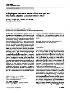
The analysis will be performed on a 128 3 64 Gaussian grid. For the experiments to be described in this section, the analysis will be done at three levels: 20, 50, and 80 kPa, as in HM. The analyzed variable is streamfunction.

FIG. 2. The locations of the (a) radiosonde and (b) satellite observations.

2) THE

OBSERVATIONS

Observation profiles are obtained from radiosondes and satellites. Their locations are presented in Fig. 2. These locations were obtained in a manner very similar to that described in HM (section 2), except that here we started with a list of the radiosonde and SATEM (i.e., satellite temperature profile) locations utilized by the operational Canadian Meteorological Centre (CMC) analysis at 0000 UTC 12 November 1998, a synoptic time chosen at random. For convenience, each observation profile was moved to the nearest point of the analysis grid. As in HM, radiosondes observe streamfunction and its horizontal derivatives at each analysis level, while satellites observe thickness between analysis levels. There are 542 radiosonde and 615 satellite profiles. For three analysis levels, these profiles yield 4878 and 1230 observations, respectively. We use the same observational-error covariance matrices for the various observations as in HM [Eqs. (1)– (3)]. The observations themselves are simulated by applying random perturbations to the (known) true state at the locations of the observations [as in Eq. (6) of HM]. Without loss of generality, the true state is taken to be zero in this study. The sets of perturbed observations to be assimilated into the ensembles of firstguess fields are generated as indicated in HM [Eq. (9)].

128

MONTHLY WEATHER REVIEW

3) ENSEMBLES

TABLE 1. The specified values of r 0 (km) and pmax , and the resulting number of batches for the experiments summarized in Fig. 3.

OF FIRST-GUESS FIELDS

Ensembles of first-guess fields, with a prescribed statistical form, are generated in a manner that is very similar to the one used to generate the initial ensemble of first-guess fields in HM (section 2). Here we use the (spectral) random-field generator described in Mitchell and Houtekamer (2000, appendix A). The separable 3D covariance structure used to generate the random field realizations is prescribed here by (i) a 3 3 3 vertical covariance matrix [HM, Eq. (4)], and (ii) a (degenerate) third-order autoregressive function, that is,

1

r0 (r) 5 1 1 ar 1

2

a2r 2 exp(2ar), 3

VOLUME 129

(9)

where a, the scale parameter, is set to 10 rad21 . b. Experiments The analysis algorithm is tested, as in HM, by examining its effect on (i) the difference between the ensemble mean and the (known) true state, and on (ii) the ensemble spread. The 50-kPa streamfunction error squared averaged over the globe is used as a measure of the error variance. Using different realizations of the ensembles of background fields and of the sets of perturbed observations, many realizations of an analysis ensemble can be produced. This evaluation technique yields statistically meaningful results about the data-assimilation algorithm itself, without requiring that data assimilation cycles be performed. 1) THE

EFFECT OF SEQUENTIAL PROCESSING OF OBSERVATION BATCHES

Inbreeding, and the nonrepresentativeness that it produces, seem to be inherent in the ensemble Kalman filter, as discussed in HM. Even with the configuration with a pair of ensembles, there is more and more dependence between the two ensembles of the pair as each batch of observations is assimilated. Consequently, the sequential algorithm might be expected to be particularly prone to inbreeding. Figure 3 summarizes a series of experiments that were performed to examine this issue. The left-hand panels of Fig. 3 show the performance of the sequential algorithm when only a single ensemble (with 16, 32, and 128 members) is used; while each corresponding righthand-side panel shows the performance obtained with a pair of ensembles having the same total number of ensemble members. Two measures of error are shown in each panel of Fig. 3: the root-mean-square (rms) difference between the ensemble mean and the true state and the rms spread in the ensemble. For all of these experiments, each batch of observations was limited to a single region and pmax , the maximum number of observations per batch, was taken to

r0

pmax

No. of batches

500 2000 5000

25 400 2500

600 69 11

be proportional to the square of r 0 (i.e., to the permitted regional area). The specific values of r 0 and pmax that were used, as well as the number of batches that were required to assimilate the 6108 available observations, are given in Table 1. For all experiments, r1 , the distance at which the correlation used in the Schur product falls to zero, was set to 5000 km. Sixteen realizations of each experiment were performed. The results of averaging over these realizations are presented in each panel of Fig. 3. The results of Fig. 3 indicate that, in general, the sensitivity of the analysis error to the size of the observation batches is rather small, both for a single ensemble and for a pair of ensembles. While the real analysis error with the smallest ensembles (upper panels of Fig. 3) exhibits a small tendency to decrease as the batch-size increases, this tendency virtually disappears for the largest ensembles (lowest panels). This is a reassuring result given the very large difference in the number of batches (Table 1) used for the experiments. A number of other aspects of the algorithm’s behavior can be discerned from Fig. 3. The single-ensemble results (left-hand panels of Fig. 3) indicate that with 16 ensemble members (upper panel of Fig. 3) the ensemble spread very substantially underestimates the ensemble mean error. As the number of ensemble members increases to 32 and then 128, the ensemble spread is seen to increase, while the ensemble mean error decreases. The result is that for the 128-member ensemble, the discrepancy between the two quantities is significantly reduced. Use of the configuration with a pair of ensembles (right-hand panels of Fig. 3) produces an ensemble spread that is much more representative of the error in the ensemble mean, but at the cost of larger ensemblemean errors for a given total number of ensemble members. These aspects of the algorithm’s performance are very much in agreement with the data-assimilation-cycle results presented in Fig. 3 of HM. With regard to the concern that the sequential algorithm might be particularly prone to inbreeding, the results of Fig. 3 indicate that, except for the smallest ensembles [O(10)], this is not a problem. What exactly constitutes a ‘‘small’’ or ‘‘large’’ ensemble is context dependent. For a system with only a few components and a few observations, one may be able to obtain a properly functioning filter with ensembles of O(10). For intermediate problems (e.g., HM or the present threelevel context), a size of O(100) seems to be sufficient. For higher-dimensional problems (e.g., for mesoscale analysis), larger ensembles would likely be required.

JANUARY 2001

HOUTEKAMER AND MITCHELL

FIG. 3. Analysis error as a function of r 0 (km), the radius of the search area for observations during the formation of regions. For these experiments, pmax , the maximum number of observations in a region, is specified to be proportional to the square of r 0 . In each panel, the rms error of the ensemble mean is indicated by the solid curve and the rms spread in the ensemble is indicated by the dashed curve. The left-hand panels are for the single-ensemble Kalman filter configuration; while the right-hand panels are for the configuration that uses a pair of ensembles. Results for different ensemble sizes are given in the upper, middle, and lower pairs of panels.

129

130

MONTHLY WEATHER REVIEW

VOLUME 129

FIG. 4. Analysis error as a function of r1 (km), the distance beyond which r is zero, for various ensemble sizes. (left) The rms spread in the ensemble, and (right) the rms error of the ensemble mean.

2) THE

EFFECT OF THE

SCHUR

PRODUCT

The effect of the Schur product is now evaluated by varying the parameter r1 for various ensemble sizes. For these experiments, each batch of observations is limited to a single region and we fix r 0 5 2000 km and pmax 5 400. With these parameters fixed, the batches are configured in the same way for all experiments. All the experiments are done using the configuration with a pair of ensembles. The results of averaging the rms analysis error over the two ensembles of the pair for eight realizations of these experiments are presented in Fig. 4. An examination of the error in the ensemble mean (right-hand panel of Fig. 4) clearly shows the benefits of increasing the ensemble size, N. In addition, it can be seen in this panel that (i) for each ensemble size there is an optimal value of r1 and (ii) this value increases as N increases. These results are very similar to those shown in Fig. 5 of HM, in which the rms analysis error was plotted, for various ensemble sizes, against the cutoff radius used in the HM algorithm. The similarity between the two figures indicates the similarity between the localizing roles played here by the correlation function used in the Schur product and in the earlier algorithm by the cutoff radius. The basis of the ensemble Kalman filter methodology is that the spread among the ensemble members be representative of the ensemble mean error. To see to what extent the current ensembles are representative, we consider the left-hand panel of Fig. 4, where the rms spread in the ensemble is shown. It can be seen that, for small distances r1 , the curves have a form similar to that exhibited in the right-hand panel of Fig. 4 by the error in the ensemble mean. A comparison of corresponding curves in the two panels indicates that, as the ensemble size increases, pairs of corresponding curves agree out to larger and larger values of r1 . For large values of r1 ,

we see that as the ensemble size increases, the ensemble mean error decreases as expected, but the ensemble spread increases. The same kind of contradictory behavior was observed in the left-hand panels of Fig. 3. It occurs here because, for values of r1 greater than the earth’s diameter, the correlation function used in the Schur product does not force a zero correlation even for points on opposite sides of the globe. The result is that we effectively obtain one global (nonlocal) analysis problem. Its dimension is fairly high (since the global background-error covariance matrix, P f , has a large number of significant eigenvalues), so a large ensemble is needed to avoid the observed inbreeding-like effects. 4. Parallel version of the algorithm A cluster of NEC SX-4 nodes, each containing up to 32 vector processors, is available at the CMC. Typical operational jobs exploit a fair number of processors on one node. To take advantage of the available computational equipment, a parallel version of the sequential algorithm has been developed. The code has been written in Fortran 77 and employs Message Passing Interface 1 (MPI-1; Gropp et al. 1994; Snir et al. 1996) for the communication between different processors. A brief discussion of the NEC SX-4 can be found in Thomas et al. (2000). To make efficient use of this computational environment, the numerical problem must be subdivided into a number of almost independent subproblems. The number of subproblems will be equal to the number of processing units and by ‘‘almost independent’’ we refer to the small amount of data that needs to be exchanged between the different processors. This amount has to be small because moving data between processors is slow compared to performing numerical operations upon data.

JANUARY 2001

HOUTEKAMER AND MITCHELL

To assess the relative importance of the different steps of the algorithm, an analysis of the number of operations involved has been performed. For the purpose of this discussion, we define a number of constants. Let Nmodel be the number of model coordinates (i.e., the number of state variables needed to describe the background field of one member of the ensemble) and let Nobs be the number of observations in the entire observation file. It is our current expectation that a configuration with Nmodel ø 10 6 , Nobs ø 10 5 and an ensemble size of N ø 10 2 could yield operationally interesting results. The most costly computations are those involving the matrix P H T . Its calculation and the subsequent solution of (8) both involve O(Nmodel Nobs N) operations. Although exploiting the sparseness of P H T leads to a reduction by perhaps a factor of 10 in numerical cost, the manipulations involving P H T still dominate any other numerical operations by several orders of magnitude. It is therefore important that the corresponding parts of the algorithm parallelize and vectorize particularly well. a. The term r + (P H T ) At any particular step of the sequential algorithm, the matrix r + (P H T ) has as many rows as there are model coordinates that can be affected by the observations being assimilated and as many columns as there are observations being assimilated at this step. In order to minimize the relative cost of the Cholesky decomposition, the number of observations in each region will be limited to some small number, say 100–1000. At each step, then, the matrix r + (P H T ) will have a huge number of rows and a fairly modest number of columns. To parallelize the computation and application of r + (P H T ), it was decided to partition the longest dimension of the matrix, which is for the model coordinate. This will be done by subdividing the model domain into a number of subdomains, so that different parts of the model space can be assigned to different processors. For the current algorithm, with its frequent computation of correlations of two quantities over the ensemble [Eqs. (2) and (3)], it did not seem advantageous to assign different ensemble members to different processors. Thus, as in Keppenne (2000), all the trial fields for some specific part of the globe are assigned to a particular processor. A strategy is therefore required for subdividing the model domain in such a way that at each step of the sequential algorithm, each processor will spend roughly the same amount of time solving (8). In the context of atmospheric data assimilation, a subdivision by vertical level or model variable is undesirable because data-assimilation codes are organized so that the interpolation operator H acts on a column containing all model variables. For instance, in the case of radiance observations, it is necessary to combine temperature and humidity information from different levels to interpolate to the observations. It was therefore decided to partition the

131

horizontal fields into a number of areas in such a way that each area would have roughly the same number of grid points. This is accomplished by partitioning the horizontal grid using a large number of fairly small tiles. Using 3 3 3 tiles leads to about 900 different tiles for a 128 3 64 horizontal grid, or over 100 tiles per processor for an eight-processor configuration. The tiles are numbered sequentially, going eastward in an inner loop and northward in an outer loop. If the number of grid points per latitude circle is not divisible by 3 (as is the case with 128 longitudes), the extra 1 or 2 longitudes are assigned to the most easterly tiles. The same procedure is followed for the most northerly ring of tiles, if the number of latitudes is not divisible by 3. The tiles are assigned one at a time to each processor in turn. This results in, say, 100 tiles scattered all over the globe being assigned to each processor. It is likely that information from many different small tiles will be needed in order to perform the analysis for a region (as defined in section 2e). This helps promote a reasonable load balance for the operations involving r + (P H T ). Consider now what data exchanges between processors are necessary for the calculation of r + (P H T ). The use of small tiles implies, from (2), that interpolated values H C fi,j corresponding to observations located on many different tiles will be required to calculate the values of r + (P H T ) associated with that portion of the trial field stored on a single processor. For this reason, the interpolated values H C fi,j are exchanged between all processors right after they are calculated. On the other hand, from (2), no exchange of trial field information is required for the computation of r + (P H T ). It is thus not necessary to exchange the haloes of the tiles between processors as would usually be done in the context of a dynamical forecast model. b. Cholesky decomposition The size of the matrix to which the Cholesky decomposition is applied can be taken as small as the number of observations in one sounding. The cost of the Cholesky decomposition of a p 3 p matrix is of order p 3 (Press et al. 1992, p. 90). There is a need for order Nobs /pmax decompositions, where pmax is the maximum number of observations in one region. The total numerical cost of the Cholesky decompositions is thus of order Nobs (with a multiplicative constant that is proportional to the square of pmax ). The subsequent backsubstitution, which needs to be performed once for each ensemble member, has an operation count of order Nobs N. Although the cost of both operations is relatively small, there is still some gain to be obtained from parallelization. Since a different linear system, (7), is solved using the Cholesky method for each region and for each ensemble of the pair, this part of the data assimilation algorithm will parallelize well if the number of available processors is equal to twice the number of regions and

132

MONTHLY WEATHER REVIEW

if the number of observations in each region is roughly constant. The result of the Cholesky method is an ensemble of vectors y i , i 5 1, . . . , N. This matrix will have to be broadcast to all processors so that it can be multiplied by the matrix r + (P H T ). As the number of observations assimilated in one pass is relatively small, as compared to Nmodel for instance, this amounts to a fairly insignificant amount of data movement. We note that the calculation of H P H T , like that of P H T , requires the values of H C fi,j , the trial field interpolated to the observations. c. Interpolation of trial fields Every processor receives those observations that are located on its tiles. For each member of the ensemble pair, it randomly perturbs each independent component of each observation profile. This yields an ensemble of perturbed observations. The next step is to interpolate the ensemble of trial fields to the observations using the operator H . The interpolated trial field values are needed for the computation of P H T and H P H T and they are broadcast to all processors. We note that for each ensemble member and each observation, exactly one interpolation needs to be performed. The total numerical cost is thus of order NNobs . This is negligible compared to the cost of computing P H T , which is of order NNobs Nmodel , unless the interpolation operator is extremely complex. Observations may, in principle, be located between grid points that have been assigned to different tiles. In that case, an extrapolation, requiring values on a single tile only, must be performed. In this way, H can be applied to a model state, without requiring the prior exchange of columns of the trial field between processors. The percentage of the observations for which extrapolation is required decreases as the size of the individual tiles increases. However, as we shall see in section 5c, increasing the size of the tiles tends to be detrimental to the load balance.

VOLUME 129

be affected by the observations into a contiguous space in memory, (b) calculate the matrix r + (P H T ), (c) multiply the matrix r + (P H T ) by the set of vectors y i,j to which it applies as in (8), and (d) copy the affected parts of the background fields back to their original locations in memory. The only one of these steps that requires information about how the tiling has been done is step 2. For step 6, each processor operates on the grid points that have been assigned to it as though they were contiguous. Steps 6a and 6d permit highly optimized matrix multiplication routines to be used for the full matrices in steps 6b and 6c. No communication between processors is required in step 6. This implies that all operations involving P H T can be executed without interruption for communication, leading to a fairly reasonable load balance. All processors synchronize, that is, wait for each other to be ready, in steps 1, 3, and 5. It is therefore important that the work assigned to all requested processors take approximately the same amount of time and that all processors be available for the algorithm during the entire execution period. 5. Performance of the parallel algorithm The parallel algorithm is intended for problems that are of operational interest. We envision implementing an ensemble Kalman filter configuration with 100 ensemble members. Each ensemble member would use some version of the CMC operational global model (GEM; Coˆte´ et al. 1998a,b) with a 192 3 96 horizontal grid and 28 vertical levels. This is the resolution currently used in the CMC ensemble prediction system. In this section, the prototype algorithm will be used to predict how much time such an application would take. We note that the time spent reading the initial trial fields and writing the final analyses is excluded from these timings. The extent to which the envisioned configuration itself would be useful is not investigated in this paper.

d. Overview of the processing of one batch To clarify how a single batch of observations is processed, we enumerate the main steps of the algorithm: 1) Communicate the characteristics of all observations to be assimilated in this batch to all processors. 2) Each processor interpolates the trial fields to the observations that are on its tiles. 3) The interpolated values are communicated to all processors. 4) The Cholesky decomposition is performed. The observations are perturbed and (7) is solved. 5) The vectors y i,j are communicated to all processors. 6) For each region the following steps are done: (a) copy the parts of the background fields that can

a. The experimental environment To obtain meaningful timings, the size of our problem must be increased. Working within the same basic experimental environment as discussed in section 3a, a convenient way to do this is to increase the number of vertical levels to 50. The same 542 radiosonde soundings (Fig. 2a), again simulating observations of streamfunction and the two wind components at each level, then correspond to 81 300 observations. Similarly, the 615 satellite profiles (Fig. 2b) yield 30 135 observations. There are thus a total of 111 435 observations to be assimilated. With 50 levels, a 128 3 64 Gaussian grid, and stream-

JANUARY 2001

133

HOUTEKAMER AND MITCHELL

function as the only analyzed variable, the number of model coordinates equals 409 600. This is smaller than the above-mentioned ‘‘realistic’’ application, which has four analysis variables at each level (and a surface pressure field), by a factor of 5. Therefore to extrapolate the timings obtained with the current prototype to the envisioned application, we must multiply by a factor of 5. For the observational-error covariance matrices, we use diagonal matrices. A diagonal vertical covariance matrix is also used in the generation of the ensemble of first-guess fields. This is done for convenience only and has no impact on the computation times. The default parameters used for the sequential algorithm will now be specified. For the formation of observation batches, the parameter r 0 is set to 500 km, the maximum number of observations allowed per region is set to 300, and a limit of 3 regions per batch is imposed. Allowing more observations per region causes the cost of the Cholesky decomposition to increase as the square of the number of observations per region, as mentioned in section 4b. Reducing the size of the observation batches increases the inbreeding effect when ensemble sizes are small, as discussed in section 3b(1). In section 5d, we will examine how changing the size of the observation batches affects the computation times. The parameter r1 is set to 4000 km. Smaller values may have to be used to reduce rank problems associated with small ensembles, as discussed in section 3b(2). Larger values of r1 may be selected for very large ensembles to reduce imbalance in the analysis increments. Larger values of r 0 or r1 would reduce the imposed sparseness of P H T and would therefore increase the cost associated with this term, which is proportional to the square of r 0 1 r1 . To partition the horizontal grid, 3 3 3 tiles are used as a default configuration. The effect of increasing the tile size will be examined in section 5c. b. Speedup The analysis code has been run with various numbers of processors, ranging from 1 to 16. For each run, the same parameters have been used, so in particular for the case with a single processor, we still used 3 3 3 tiles. (While in fact there is no reason to introduce tiles with only one processor.) For an operational application, an attempt would be made to determine the most suitable tile size for any given number of processors. A timing profile (not shown) indicated that for the case with a single processor about 95% of the time is spent on the operations involving P H T (section 4d, step 6). It is encouraging to see such a high percentage because the algorithm was designed so that the treatment of this term would vectorize and parallelize particularly well. The Cholesky decomposition takes only 2% of the time, but we note that the relative amount of time spent on this computation can be controlled by allowing more or less observations per region. We note that for all

TABLE 2. The performance of the parallel program on a NEC SX4 for a pair of 50-member ensembles and different numbers of processors. The number of millions of floating point operations per second (Mflop s21 ) is given per processor. The total execution time (s) is given as real time. The speedup is the speed-gain factor for real time with respect to the single-processor configuration. Processors

Mflop s21

Real time (s)

Speedup

1 2 8 12 16

1767 1700 1522 1401 1371

1450 770 215 158 118

1.00 1.88 6.74 9.18 12.28

experiments with the parallel algorithm, the mean vector length averaged over all processors exceeded 210. This is close enough to the machine maximum of 256 to yield good performance. Benchmark results, for various numbers of processors, are shown in Table 2. It can be seen that the singleprocessor configuration runs at 1.77 Gflop s21 . The optimal value on this computer, for an extremely wellcoded algorithm, would be about 2 Gflop s21 . For the case with one processor, only a small improvement on our current timings could be gained by code optimization. It can be seen in Table 2 that the flop rate averaged over all processors goes down as the number of processors increases. This is probably mainly due to the time required to exchange information between processors during the algorithm, which may include idle time when all but one of the processors have to wait until some specific one has completed its numerical calculations. The real-time column in Table 2 shows the total time that was required for the program to be executed on the computer. This time is evidently smaller when a larger number of processors is used. With 16 processors, the program is executed in 118 s. Multiplying by a factor of 5, gives an estimate of 10 min for the ‘‘realistic’’ application. This is similar to the time traditionally taken by the operational analysis at the CMC. From Table 2, we obtain an estimate of 2 h on one processor, which might be too long. In the speedup column of Table 2 we show by what factor the real time decreased as a result of using more processors. Ideally the speedup should equal the number of processors. In fact when we first tested the software on a different computer that did not have vector processors, the term P H T was even more dominant and we obtained a nearly perfect speedup. Unfortunately the corresponding real time was unacceptable. The results in this section, while encouraging in general, are specific to the type of computer for which this code was written and optimized. The benchmark would have to be redone for any other computational environment for which the ensemble Kalman filter was being considered. Nevertheless an underestimate of the real time for another computer can be obtained by assuming a computational cost of order Nmodel Nobs N, considering

134

MONTHLY WEATHER REVIEW

TABLE 3. The load imbalance is quantified for different tile sizes. For each processor the total number of Gflops was counted. The lowest and the highest values are listed. A big difference between these values leads to a longer real time. Gflop count Tile size

Lowest

Highest

Real time (s)

3 3 3 3 3 3

201 202 186 188 151 129

228 214 236 229 282 304

158 152 167 169 251 238

3 4 6 8 10 12

3 4 6 8 10 12

the optimal Gflop rate for that computer and extrapolating from the results in Table 2. c. Tiling of the sphere As the tile size increases, it becomes less likely that, at any step of the sequential algorithm, all processors will be responsible for a similar number of grid points that can be affected by the observations being assimilated. In Table 3 we show how the real time increases when larger tiles are used. All of these experiments were performed using 12 processors. It can be seen that the current algorithm has a fairly constant numerical performance for tiles of size 8 3 8 or smaller. Note that both 128 and 64 are divisible by 8 so that the number of grid points per processor differs by at most 64 (i.e., one tile). For tiles of 10 3 10, the performance of the algorithm deteriorates substantially and some processors have to do much more work than others. The Gflop count for the busiest processor is 282, the most idle one has a workload of only 151, while the other processors have Gflop counts that fill in the range between these two extremes. This imbalance directly translates into a much increased real time. We note that the total Gflop count, summed over the 12 processors, had a very nearly constant value of 2509.3 Gflop. This occurs because, when it comes to calculations involving P H T , only those grid points are considered that are close enough to the center of a region that they may be affected. The number of such grid points is not a function of the size of the tiles. We remark that the use of small tiles implies that a relatively large fraction of the observations will be near the edge of a tile. For these observations, the calculation of the trial field value at the observation location will incur an undesirable extrapolation error. The use of larger tiles reduces the fraction requiring extrapolation. However for larger tiles, more advanced tile-forming algorithms are desirable so that the load imbalance is minimized, for example, algorithms that ensure that all processors are assigned the same number of grid points or that take account of the observation density when forming tiles. When a very large number of processors (say over 100) is being used, load balance problems may become very serious.

VOLUME 129

TABLE 4. Effect on the performance of the parallel algorithm of changing the batch size. All experiments are performed with 4 3 4 tiles and, as in Table 3, with 12 processors. In addition to the lowest and highest Gflop count, the total number of Gflops (over all processors) is also shown. Note that with r 0 5 2 km, each region contains exactly one sounding. Obs per Gflop count region No. of r0 (km) (max) batches Lowest Highest Total 2 500 1000

150 300 1200

401 218 90

161 202 250

168 214 287

1980.2 2509.3 3169.9

Real time (s) 126 152 222

For the assimilation into a fine-mesh model of limbsounding data, for example, global positioning system/ meteorology data (Rocken et al. 1997), a different tiling strategy may have to be adopted because the interpolation operator H would require many columns of trial field values. d. Impact of changing the batch size The effect of changing the size of the observation batches is illustrated in Table 4. Three different specifications of the batch size parameters are considered. All experiments are performed with 4 3 4 tiles and, as in the previous experiments in this section, a limit of three regions per observation batch is imposed. The configuration with r 0 5 500 km and a maximum of 300 observations per region is the baseline configuration, for which results have already been shown in Table 3. As can be seen in Table 4, when r 0 is reduced to 2 km, 401 (rather than 218) batches are required to assimilate the 1157 available soundings. The total number of floating-point operations decreases by 21% as compared to the baseline configuration. When r 0 and the maximum number of observations per region are increased to 1000 km and 1200, respectively, the number of batches drops to 90. The total number of floatingpoint operations increases by 26%, as compared to the original configuration. Most of the observed variation in the number of floating-point operations is due to changes in the sparseness of P H T . As indicated in section 5a, the cost associated with this term is proportional to the square of r 0 1 r1 . With r1 5 4000 km, our changes to r 0 have the effect of decreasing this quantity by 21% and increasing it by 23%, as compared to the baseline configuration. It can be seen that there is an increase in the load imbalance as the batch size increases. This is largely due to the increased size of the matrix problem, (7), associated with larger batches. With a specified maximum of three regions per batch, at most six (of the 12 available) processors are needed for the Cholesky decompositions. The execution times are not strictly proportional to the observed variation in the number of floating-point operations, due mostly to the increase with batch size of the load imbalance. Reducing r 0 to

JANUARY 2001

HOUTEKAMER AND MITCHELL

2 km is seen to reduce execution times by 17%, as compared to the baseline configuration, whereas allowing larger batches increases execution times by 46%. This confirms the advantages of limiting the size of the observation batches. 6. Summary and concluding discussion The ensemble Kalman filter uses the nonlinear forecast model to transport the forecast-error covariances from one analysis time to the next. It therefore constitutes, not only an approximation to, but also a nonlinear extension of, the standard Kalman filter. It represents a promising approach toward the goal of developing a Kalman filter–based algorithm for atmospheric data assimilation. However, for the technique to be feasible in an operational setting, a computationally efficient analysis algorithm is required. In this paper, we have proposed and tested a prototype having a number of desirable properties (enumerated in section 1). It is based on the algorithm of Evensen (1994), as modified by HM. Although that earlier algorithm performed well when assimilating the approximately 1000 observations available at each analysis time in HM, it was recognized there that it ‘‘would become prohibitively expensive if the data were very dense.’’ Given that in an operational environment the number of available observations may exceed 100 000 (6-h period)21, this is a potentially serious problem. To address this issue, we have exploited the fact that a properly functioning ensemble Kalman filter produces representative ensembles not only of the short-range forecasts (which serve as background fields for the analysis), but also of the analyses themselves. The ensembles of analyses can provide estimates of the analysiserror covariances. Therefore if the observations are organized into batches, we can assimilate the batches sequentially, using the analyzed fields resulting from the assimilation of one batch as background fields for the assimilation of the next batch. The evolution of the ensemble of background fields at each step provides a measure of the improving quality of the background fields as more and more batches of observations are assimilated. As shown in Fig. 3, this technique works very well: the quality of the analysis is found to vary little, if a given set of observations is partitioned into say 10 or 600 batches (except when the ensemble is extremely small). Sequential processing of batches of observations is a standard technique in Kalman filter theory. However, this strategy has not as yet been applicable in operational atmospheric-data-assimilation algorithms. These algorithms generally employ parameterized representations of the background (i.e., forecast) error and, in the context of these algorithms, there is no way of updating the required background-error statistics after a given batch of observations is assimilated. The cutoff radius, introduced in HM, eliminated the

135

need to have to estimate the small correlations associated with remote observations and alleviated the rank problem associated with the ensemble Kalman filter. However, it was likely a source of noise, and in a primitive equations context would likely produce imbalance. In the current algorithm, localization is achieved in a different way: we now use a Schur (elementwise) product of the covariances calculated from the ensemble and a correlation function having local support (Gaspari and Cohn 1999). This filters the small correlations associated with remote observations and, since the correlation function is smooth and monotonically decreasing, produces smooth analysis increments. The effect of localization is to increase the effective number of ensemble members. For example, one can think of a correlation function that has significant amplitude only over 10% of the globe as effectively multiplying the number of ensemble members by a factor of 10. As shown in Fig. 4 (right-hand panel), for each ensemble size there is an optimal length scale for the Schur product correlation function and this optimal length scale increases as the ensemble size increases. [Analogous results relating to the cutoff radius were presented in HM (Fig. 5).] Thus as the number of ensemble members increases and as the noise in the estimate of weak distant correlations diminishes, we can reduce the effect of the Schur product by increasing the length scale of the correlation function. One attractive feature of the ensemble Kalman filter technique is the possibility of performing the different ensemble forecasts on different processors, if multiple processors are available (Evensen 1994). It is important to realize that in an operational context these time integrations are not time critical. One can start preparing the required short-range forecasts as soon as the preceding analyses are available. In the case of a 6-h dataassimilation cycle, approximately 4 h might be available to execute this step. To complement the suitability of the forecast step for parallel computation, a parallel version of the sequential ensemble Kalman filter has been presented in section 4. Its operation count is proportional to the number of observations, the number of model coordinates, and the number of ensemble members. It yields analyses that are identical regardless of the number of processors utilized, except for an extrapolation of trial field values near the edges of the tiles assigned to different processors. These extrapolations could be avoided by using a sequence of three slightly shifted tilings, where for each tiling only those observations not requiring extrapolation are assimilated. A possible alternative parallel algorithm would be one where the assimilation problem for different grid points (or grid volumes) is done independently and made feasible by introducing a cutoff radius or another data selection procedure (e.g., HM, Stobie 2000). Because of the independence, such an algorithm is embarrassingly parallel and yields a nearly perfect speedup. The data selection results in a significant saving for operations

136

MONTHLY WEATHER REVIEW

involving P H T . However to ensure smooth analyses, the matrix problems being solved for neighboring grid volumes must be almost the same and a fairly large number of observations must be selected (Cohn et al. 1998; Steinle et al. 1999). One notable difference that appears when comparing the ensemble Kalman filter with other Kalman filter implementations (e.g., Lyster et al. 1997) is the way covariances are computed. The ensemble Kalman filter computes covariances directly from the ensemble, using (2) and (3), when they are required. In practice, the sequential algorithm only uses fairly small matrices at any particular time, so that the memory requirement is fairly modest. The current algorithm has been developed specifically for the purpose of performing global, synoptic-scale, atmospheric analyses at CMC. The dependence of the results on various tunable parameters of the algorithm has been examined. Even within the limited scope of this objective, various choices of these parameters could be selected depending on external constraints, such as the available computing time and the acceptable approximation error. For other data-assimilation applications and environments, other algorithms may be more suitable. However, we feel that the current study, as well as the recent study by Keppenne (2000), strongly suggests that application of the ensemble Kalman filter, with a realistic model, is now feasible on modern supercomputers. In an operational context, observations valid at a given time arrive fairly continuously over a period of several hours. A cutoff time of, say, 3 h might be allowed for the receipt of the observations. This suggests that, if execution of the sequential algorithm begins upon arrival of the first observations, several hours would be available for the assimilation. In that case, even the single-processor configuration would be fast enough for the currently envisioned 100-member application. Alternatively, using several processors, one could decide to assimilate a significantly larger volume of remotely sensed data. In the context of remotely sensed data, it may be necessary to account for horizontal correlations. One option would be to sample systematic problems with the interpolation to the observations by systematically using different versions of these interpolation operators for different ensemble members. The method used here to evaluate the sequential algorithm did not involve the use of a forecast model. While this method had the advantage of allowing the analysis algorithm to be studied in isolation, it required that we assume an externally prescribed form for the forecast-error covariances. There is the possibility that the assumed spectrum may have had an impact on some aspects of the algorithm’s performance. Also, we were unable to study issues involving interactions between the model dynamics and the analysis algorithm, for example, the balance of the analysis increments. To investigate these issues and to study some other remaining

VOLUME 129

questions, in particular concerning the required ensemble size and the parameterization of model error, we intend to combine the sequential analysis algorithm with a primitive equations model. Acknowledgments. We thank Stephen Cohn and Richard Me´nard for suggesting the Schur product with a compactly supported correlation function in place of the cutoff radius that we had employed in HM. We thank Luc Fillion, whose constructive criticism of the HM algorithm provided the impetus for this study. We express our appreciation to Michel Valin for introducing us to MPI and for suggestions that improved the performance of the parallel algorithm. We thank Ste´phane Laroche and Monique Tanguay for their helpful internal reviews of the manuscript. The comments of the two anonymous reviewers helped us clarify a number of points and sharpen the focus of the paper. REFERENCES Anderson, B. D. O., and J. B. Moore, 1979: Optimal Filtering. Prentice-Hall, 357 pp. Anderson, J. L., and S. L. Anderson, 1999: A Monte Carlo implementation of the nonlinear filtering problem to produce ensemble assimilations and forecasts. Mon. Wea. Rev., 127, 2741–2758. Andersson, E., J. Pailleux, J.-N. The´paut, J. R. Eyre, A. P. McNally, G. A. Kelly, and P. Courtier, 1994: Use of cloud-cleared radiances in three/four-dimensional variational data assimilation. Quart. J. Roy. Meteor. Soc., 120, 627–653. Brown, R. G., 1983: Introduction to Random Signal Analysis and Kalman Filtering. Wiley and Sons, 347 pp. Burgers, G., P. J. van Leeuwen, and G. Evensen, 1998: Analysis scheme in the ensemble Kalman filter. Mon. Wea. Rev., 126, 1719–1724. Cohn, S. E., and D. F. Parrish, 1991: The behavior of forecast error covariances for a Kalman filter in two dimensions. Mon. Wea. Rev., 119, 1757–1785. , A. da Silva, J. Guo, M. Sienkiewicz, and D. Lamich, 1998: Assessing the effects of data selection with the DAO physicalspace statistical analysis system. Mon. Wea. Rev., 126, 2913– 2926. Coˆte´, J., J.-G. Desmarais, S. Gravel, A. Me´thot, A. Patoine, M. Roch, and A. Staniforth, 1998a: The operational CMC–MRB Global Environmental Multiscale (GEM) model. Part II: Results. Mon. Wea. Rev., 126, 1397–1418. , S. Gravel, A. Me´thot, A. Patoine, M. Roch, and A. Staniforth, 1998b: The operational CMC–MRB Global Environmental Multiscale (GEM) model. Part I: Design considerations and formulation. Mon. Wea. Rev., 126, 1373–1395. Derber, J. C., and W.-S. Wu, 1998: The use of TOVS cloud-cleared radiances in the NCEP SSI analysis system. Mon. Wea. Rev., 126, 2287–2299. , D. F. Parrish, and S. J. Lord, 1991: The new global operational analysis system at the National Meteorological Center. Wea. Forecasting, 6, 538–547. Evensen, G., 1994: Sequential data assimilation with a nonlinear quasi-geostrophic model using Monte Carlo methods to forecast error statistics. J. Geophys. Res., 99 (C5), 10 143–10 162. , 1997: Advanced data assimilation for strongly nonlinear dynamics. Mon. Wea. Rev., 125, 1342–1354. , and P. J. van Leeuwen, 1996: Assimilation of Geosat altimeter data for the Agulhas current using the ensemble Kalman filter with a quasigeostrophic model. Mon. Wea. Rev., 124, 85–96. Gaspari, G., and S. E. Cohn, 1999: Construction of correlation func-

JANUARY 2001

HOUTEKAMER AND MITCHELL

tions in two and three dimensions. Quart. J. Roy. Meteor. Soc., 125, 723–757. Gropp, W., E. Lusk, and A. Skjellum, 1994: Using MPI. Portable Parallel Programming with the Message-Passing Interface. Scientific and Engineering Computation Series, The MIT Press, 307 pp. Horn, R. A., and C. R. Johnson, 1985: Matrix Analysis. Cambridge University Press, 561 pp. Houtekamer, P. L., and H. L. Mitchell, 1998: Data assimilation using an ensemble Kalman filter technique. Mon. Wea. Rev., 126, 796– 811. , and , 1999: Reply. Mon. Wea. Rev., 127, 1378–1379. Jiang, S., and M. Ghil, 1993: Dynamical properties of error statistics in a shallow-water model. J. Phys. Oceanogr., 23, 2541–2566. Keppenne, C. L., 2000: Data assimilation into a primitive-equation model with a parallel ensemble Kalman filter. Mon. Wea. Rev., 128, 1971–1981. Lyster, P. M., S. E. Cohn, R. Me´nard, L.-P. Chang, S.-J. Lin, and R. G. Olsen, 1997: Parallel implementation of a Kalman filter for constituent data assimilation. Mon. Wea. Rev., 125, 1674–1686. McNally, A. P., J. C. Derber, W. Wu, and B. B. Katz, 2000: The use of TOVS level-1b radiances in the NCEP SSI analysis system. Quart. J. Roy. Meteor. Soc., 126, 689–724. Miller, R. N., E. F. Carter Jr., and S. T. Blue, 1999: Data assimilation into nonlinear stochastic models. Tellus, 51A, 167–194.

137

Mitchell, H. L., and P. L. Houtekamer, 2000: An adaptive ensemble Kalman filter. Mon. Wea. Rev., 128, 416–433. Press, W. H., S. A. Teukolsky, W. T. Vetterling, and B. P. Flannery, 1992: Numerical Recipes in FORTRAN. The Art of Scientific Computing. 2d ed. Cambridge University Press, 963 pp. Rocken, C., and Coauthors, 1997: Analysis and validation of GPS/ MET data in the neutral atmosphere. J. Geophys. Res., 102 (D25), 29 849–29 866. Snir, M., S. W. Otto, S. Huss-Lederman, D. W. Walker, and J. Dongarra, 1996: MPI. The Complete Reference. Scientific and Engineering Computation Series, The MIT Press, 336 pp. Steinle, P. J., B. R. Harris, and R. S. Seaman, 1999: Variational data assimilation at the Bureau of Meteorology. Preprints, 13th Conf. on Numerical Weather Prediction, Denver, CO, Amer. Meteor. Soc., 33–36. Stobie, J., 2000: An efficient objective analysis system for parallel computers. Proc. 2d Int. Conf. on Reanalyses, Reading, United Kingdom, World Climate Research Programme, WMO/TD No. 985, 103–106. Thomas, S. J., M. Desgagne´, and M. Valin, 2000: High-resolution weather forecasting: A teraflop sustained on RISC/cache or vector processors. High Performance Computing Systems and Applications, A. Pollard, D. J. K. Mewhort, and D. F. Weaver, Eds., Kluwer Academic, 289–299. van Leeuwen, P. J., 1999: Comments on ‘‘Data assimilation using an ensemble Kalman filter technique.’’ Mon. Wea. Rev., 127, 1374– 1377.