A Sequential Sampling Scheme for Detecting Infestation Levels of. Tracheal Mites (Heterostigmata: Tarsonemidae) in Honey Bee. (Hymenoptera: Apidae) ...
APICULTURE AND SOCIAL INSECTS
A Sequential Sampling Scheme for Detecting Infestation Levels of Tracheal Mites (Heterostigmata: Tarsonemidae) in Honey Bee (Hymenoptera: Apidae) Colonies MARYANN T. FRAZIER, JENNIFER FINLEY, WILLIAM HARKNESS,1
AND
EDWIN G. RAJOTTE
Department of Entomology, The Pennsylvania State University, 501 ASI Building, University Park, PA 16802
J. Econ. Entomol. 93(3): 551Ð558 (2000)
ABSTRACT The introduction of parasitic honey bee mites, the tracheal mite, Acarapis woodi (Rennie) in 1984 and the Varroa mite, Varroa jacobsoni, in 1987, has dramatically increased the winter mortality of honey bee, Apis mellifera L., colonies in many areas of the United States. Some beekeepers have minimized their losses by routinely treating their colonies with menthol, currently the only Environmental Protection Agency-approved and available chemical for tracheal mite control. Menthol is also expensive and can interfere with honey harvesting. Because of inadequate sampling techniques and a lack of information concerning treatment, this routine treatment strategy has increased the possibility that tracheal mites will develop resistance to menthol. It is important to establish economic thresholds and treat colonies with menthol only when treatment is warranted rather than treating all colonies regardless of infestation level. The use of sequential sampling may reduce the amount of time and effort expended in examining individual colonies and determining if treatment is necessary. Sequential sampling also allows statistically based estimates of the percentage of bees in standard Langstroth hives infested with mites while controlling for the possibility of incorrectly assessing the amount of infestation. On the average, sequential sampling plans require fewer observations (bees) to reach a decision for speciÞed probabilities of type I and type II errors than are required for Þxed sampling plans, especially when the proportion of infested bees is either very low or very high. We developed a sequential sampling decision plan to allow the user to choose speciÞc economic injury levels and the probability of making type I and type II errors which can result inconsiderable savings in time, labor and expense. KEY WORDS Apis mellifera, honey bee, Acarapis woodi, tracheal mite, sequential sampling, bee mortality
BEFORE THE INTRODUCTION of the tracheal mite Acarapis woodi (Rennie), a 10% loss of colonies during the winter was considered normal in Pennsylvania apiaries. During the late 1980s and early 1990s, before the widespread presence of the Varroa mite, Varroa jacabsoni, Pennsylvania beekeepers experienced unusually high winter mortality of honey bee, Apis mellifera (L.), colonies even during relatively mild winters. In a 1988 Ð1989 study, the average winter loss of colonies in uninfested beekeeping operations was 11%, whereas the average loss in tracheal mite infested operations was 31.4% (Frazier et al. 1994). Losses within individual apiaries were as high as 100%. This increase in colony mortality in Pennsylvania is similar to reports of 30 Ð50% in New York (Scott-Dupree and Otis 1989), 50 Ð70% in Northern Florida (Gruszka 1987), and an average of 40% in Washington commercial beekeeping operations (Anonymous 1989). This situation has threatened the supply of bees available for pollination throughout the United States and continued losses could be disastrous for the growers of bee-pollinated crops, as well as for beekeepers. En1 Department of Statistics, The Pennsylvania State University, University Park, PA 16802.
suring the survival of a strong beekeeping industry is important to agriculture. Beekeepers are treating their colonies with menthol, which reduces tracheal mite infestation levels (Herbert et al. 1987). However, menthol treatments are relatively expensive, costing approximately $2.75 per colony. In addition, the application is time-consuming and labor-intensive, interferes with honey harvesting, and can be ineffective in the cooler temperatures of the northeast where the sublimation of the menthol crystals can be retarded. The increased costs of buying and applying chemical controls are passed on to growers of bee-pollinated crops in the form of increased pollination fees. These in turn may be passed on to consumers. In addition, the regular use of menthol or other chemical treatments may delay the natural selection of honey bee colonies that are better adapted to survive tracheal mite infestations. It is thought that the recovery of the European beekeeping industry from tracheal mite infestations was because of genetically based changes in the resistance of the bees (Morgenthaler 1931; Adam 1968, 1987). The routine use of menthol, regardless of infestation levels, may increase the possibility that tracheal mites will develop resis-
0022-0493/00/0551Ð0558$02.00/0 䉷 2000 Entomological Society of America
552
JOURNAL OF ECONOMIC ENTOMOLOGY
tance to menthol. Routine treatment also increases the risk of contaminating the honey crop with menthol. Ideally, chemical treatments should be applied only when the mite infestation reaches a level that will cause economic damage (economic threshold). There is some debate over the level at which tracheal mites cause economic damage. Rennie (1922) and Morgenthaler (1931) reported this level to be 50% of the bees in a colony infested, and Bailey (1958, 1961) reported 30%. More recently, Eischen et al. (1989) reported that an infestation level ⬎25% was likely to cause economic damage. Many factors may contribute to these reported differences (e.g., environmental conditions, honey bee genotype). Regardless of the disputed economic threshold levels, a practical sampling procedure that will estimate the level of infestation with any reasonable degree of conÞdence, has not been developed. The determination of sampling regimes for colonies, apiaries, and beekeeping operations, has not yet been described in acceptable statistical terms. Therefore, the decision whether to treat colonies or apiaries for tracheal mites, based on infestation levels, could not be made with adequate certainty in the past. Moreover, the procedures used were time-consuming and not responsive to apparent infestation intensity. The ability to estimate tracheal mite populations quickly and accurately is important for beekeepers trying to determine whether treatment of colonies is necessary, and for researchers studying the population dynamics and control of the mite. Many state regulatory agencies have taken on the responsibility of diagnosing tracheal mites infestations. Because of labor-intensive, time-consuming detection procedures, and limited resources, these regulatory agencies for the most part are restricted to looking at composite apiary samples and determining the presence or absence of mites, rather than providing any quantitative information concerning infestation levels. Attempts have been made to improve the accuracy and ease of determining tracheal mite populations by improving both sampling procedures (Calderone and Shimanuki 1992) and detection techniques (Colin et al. 1979, Peng et al. 1985, Smith et al. 1987). In the current study, sequential sampling plans are described, formulas are given, and their use is illustrated on samples to classify tracheal mite infestation. Sequential Sampling Plans. Sequential sampling plans classify populations into dichotomous groups through testing hypotheses about a characteristic (parameter) of the populations. Low infestation levels of A. woodi do not adversely affect colonies, whereas high infestation levels often result in the death of colonies (Tomasko and Finley 1990). In this study, the populations of bees in colonies are described as having either high or low tracheal mite infestations, according to the proportion (p) of bees infested. Although our study uses a mite prevalence score, some investigators feel the parasite load score, or the average number of mites per bee, is a more accurate indicator of a infes-
Vol. 93, no. 3
tation level; however, Calderone and Shimanuki (1995) have shown that mite prevalence values and parasite load scores are highly correlated. In contrast to sequential sampling plans, ordinary sampling plans are based on a Þxed sample size. The sampling methodology currently in use generally involves samples varying in size from 20 to 50 bees (Calderone and Shimanuki 1992). Typically, the samples are composite apiary samples made up of a few bees from each colony in the apiary. On the average, sequential sampling plans require fewer observations (bees) to reach a decision about H1 and H2 than required for “Þxed plans,” especially when the proportion (p) of infested bees is either very low or very high. Therefore, sequential sampling plans are potentially more efÞcient in terms of sampling effort. Onsager (1976) has presented the rationale for sequential sampling, given formulas for these plans, and has discussed some applications to sampling for insect pests. The use of sequential sampling has become increasingly widespread since WatersÕ (1955) description of the use of such procedures in biological populations. For example, see implementations of these plans by Foster et al. (1982), McAuslane and Ellis (1987), and Shields et al. (1991) to characterize corn rootworm populations. Twenty different sequential sampling decision tables have been generated and are available (Tomasko et al. 1993). Additional tables can be generated using the formulas given by Onsager (1976). Materials and Methods We established two hypotheses: H1: p ⫽ p1 and H2: p ⫽ p2. Samples of bees were examined individually for presence or absence of infestation. After each bee was examined, one of three possible decisions was made, based on the cumulative number (y) of infested bees found in the Þrst (n) bees looked at: (1) conclude H1, asserting that the proportion of infested bees in the colony is p1or less than p1, (2) conclude H2, asserting that the proportion of infested bees is p2 or greater than p2, or (3) continued examination of bees because the results were inconclusive about H1 and H2. In this study, p1 and p2 are chosen to reßect the investigatorÕs estimation of truly high or low infestation levels. Infestation levels between p1 and p2 indicate that there has not been enough infestation obtained through sampling to make a decision, so more samples are needed. Thus, the sample size required to make a decision is variable and could be based on the colony infestation level, the selected levels of p1 and p2, and the degree of accuracy selected by the decisionmaker. In addition, p values were selected based on samples collected from the inner cover and top bars of the hive. Tracheal mite infestation levels within a colony are known to vary depending on season and location within the hive (Calderone and Shimanuki 1992). If samples are taken at different times of the year and different places within the hive, p1 and p2 could be adjusted to reßect the relationship between
June 2000
FRAZIER ET AL.: SEQUENTIAL SAMPLING SCHEME FOR TRACHEAL MITES
tracheal mite infestations in different parts of the colony and different times with the true infestation level of the colony. Along with the selection of p1 and p2 the decisionmaker must select acceptable levels of type I and type II errors. A type I error is committed when an infestation is classiÞed as above the economic threshold when it is really below it, and a type II error is made when an infestation is classiÞed as below the economic threshold when it is really above. The probabilities of type I and type II errors are a part of the sequential sampling design. In the case of tracheal mites, the cost of making a type I error is not as serious as making a type II error in economic terms. Type I and type II errors can be set by the decision-maker to reßect the consequences (economic or otherwise) of these errors. The present sequential sampling scheme was designed around detecting mite infestations at a speciÞc point in time. Decision-makers must use these data in light of honey bee and mite biology at that particular time to determine if treatment is necessary. Field and Laboratory Experimental Procedure. This sequential sampling scheme was developed as part of a larger experiment in which menthol control tactics were compared (Tomasko et al. 1990). In this experiment, 72 colonies belonging to a commercial beekeeper were used to develop an improved menthol delivery system. One-half (36) of these colonies had high pretreatment levels of tracheal mite infestation (35 or more bees of 50 infested). The remaining onehalf (36) had a low level of infestation (15 or fewer bees of 50 infested). These were divided equally into two menthol treatment groups (an early treatment and late treatment), and a control group. The 72 colonies were then divided equally into four apiaries (yards). An equal number of high infested and low infested colonies were placed in each apiary. A random numbers decision table was used to assign each colony to a treatment or control. The 24 colonies in the early treatment were treated with 50 g of menthol on 11 September 1989. Colonies assigned to late menthol treatments received the same amount of menthol, on 13 October 1989. All colonies were treated with bioclohexylammonium fumigillin (Fumidil-B, Rhone Merieux, Canada, Victoriaville, QC, Canada, 200 mg[AI] per colony) to reduce the effect of nosema disease. Hygrothermographs were placed in each of the four apiaries to record daily temperature and humidity. Samples of 50 bees were collected from the early treatment and control colonies on 13 October, 1 mo after treatment. Samples from the late treatments were collected on 14 November 1 mo after treatment. Subsequent samples were collected from all colonies on the following dates in 1990: 19 January, 1 March, and 17 April. All bee samples were collected from the inner cover or the outside frames from the upper most hive box containing bees and preserved in 70% EtOH. Samples were examined for tracheal mites using the method described by Shimanuki and Knox (1991).
553
Generation and Validation of Sequential Sampling Decision Plan. Using the formulations given by Onsager (1976), the sequential probability ratio test of H1: p ⫽ p1 versus H2: p ⫽ p2 with probabilities of type I and type II errors ␣ and  respectively, is given by the following: (1) accept H1, if y ⫽ a1 ⫹ bn, (2) reject H1 (accept H2), if y ⫽ a2 ⫹ bn, (3) continue sampling, if a1 ⫹ bn ⬍ y ⬍ a2 ⫹ bn,
冉 冊冒 冉 冊 冉 冊冒 冉 冊冒 冉 冊
where a1 ⫽ ⫺ln a2 ⫽ ln and b ⫽ ln
1⫺␣ 
ln
p2q1 , p1q2
1⫺ ␣
ln (p2q1/p1q2)
q1 q2
p2q1 ; q ⫽ 1 ⫺ p1. p1q2 1
ln
It is assumed that p1 ⬍ p2 and that (y) is the number of infested bees among the Þrst (n) examined. If, for the sake of convenience, bees are examined in groups of size m ⬎ 1, then the only change in these formulas consists of replacing (n) with (mn), where (n) is the number of groups (of size m) examined. Example: Let ␣ ⫽ 0.10,  ⫽ 0.05, H1: p ⫽ p1 ⫽ 0 .1, H2: p ⫽ p2 ⫽ 0.3. The sequential sampling plan consists of examining bees one at a time. In this case, a1 ⫽ ⫺2.141, a2 ⫽ 1.668, b ⫽ 0.1862 One accepts H1 if after examining (n) bees, y ⫽ ⫺2.141 ⫹ 0.1862n, rejects H1 if y ⫽ 1.668 ⫹ 0.1862n and continues sampling another bee if ⫺2.141 ⫹ 0.1862n ⬍ y ⬍ 1.668 ⫹ 0.1862n. In addition to the basic output of sequential sampling plans, some other calculations may be useful. Let LP be the “level of probability” of the test, meaning “the chance that the hypothesis H1 is accepted.” For example, the probability of a type I error (rejecting H1 when H1 is true) is ␣ and so the chance that H1 is accepted when H1 is true is LP ⫽ 1⫺␣. If p ⫽ 0.00, then LP ⫽ 1.00, and when H2 is true, LP ⫽ . Also, LP ⫽ 0.000 when p ⫽ 1. One other value of LP can be obtained: for p ⫽ b (the slope of the two lines), LP ⫽ a2/(a2 ⫺ a1); and it can be shown that (always) p1 ⬍ b ⬍ p2. Also of interest are average sample numbers, which are the long-run average sample sizes to reach decisions about H1 and H2. The average sample numbers depend on the true proportion (p). Formulas for level of probability and average sample numbers (for Þve special values noted above) and their values for the sequential sampling plan for H1: p ⫽ 0.10, H2: p ⫽ 0.30, ␣ ⫽ 0.10, and  ⫽ 0 .05 are given in Table 1. The chance that H1: p ⱕ 0.10 is accepted when in fact the proportion of bees with tracheal mite infestation is b ⫽ 0.1862 is LP ⫽ 0.44 and so the chance that H1 is rejected (and H2: p ⫽ 0.30 is accepted) is 1Ð 0.44 ⫽ 0.56; the chance that H1 is rejected when p ⫽ p2 ⫽ 0.30 is 1Ð 0.05 ⫽ 0.95 ⫽ 1⫺. As for the expected number of bees that need to be examined, from above it is seen that if H1 is true (p ⫽ p1), then ⬇20 bees will be examined; if H2 is true (p ⫽ p2), then 13 bees will need to be looked at (on the average). For the
554
JOURNAL OF ECONOMIC ENTOMOLOGY
Table 1. Sequential sampling plan for H1: p < 0.10, H2: p > 0.30, ␣ ⴝ 0.10, and  ⴝ 0.05 p⬘ 0 p1 b p2 1
LP
ASN
Formula
Value
Ñ (1 ⫺ ␣)
1.00 0.90 0.44 0.05 0.00
 Ñ
Formula (1 ⫺ ␣)(a1 ⫺ a2)
(a1 ⫺ a2)⫹a
Value
Table 2. Example decision table, where P < 0.10 (10%) versus P > 0.30 (30%); ␣ ⴝ 0.10 and  ⴝ 0.05 No. beesa
11.5 20.4 23.5 13.0 2.0
1 2 3 4 5 6 7 8 9 10 11 12 13 14 15 16 17 18 19 20 21 22 23 24 25 26 27 28 29 30 31 32 33 34 35 36 37 38 39 40 41 42 43 44 45 46 47 48 49 50
From Onsager (1976). LP, level of probability; ASN, average sample number.
sake of comparison, if a Þxed sample plan were used, the requisite sample size for testing H1: p ⫽ 0.10 versus H2: p ⫽ 0.30, with ␣ ⫽ 0.10 and  ⫽ 0.05 would be 33. Validation. The 70 samples collected from menthol experiment colonies in January (includes early, late, and controls treatments, and high and low infestations) were used to illustrate the sequential sampling plan developed here. As individual bees (individuals in the group of 50) were examined under the microscope, detailed records were kept of whether the bee was infested and of the ordinal position of the bee in the group being examined. The data collected and recorded were used to validate the sequential sampling decision tables. Sequential sampling plans for testing hypotheses about the proportions (p) of infested bees are based on the number (y) of positive (infested) bees found in (n) bees examined. The variable (y) is assumed to have a binomial distribution and this will be the case if: (1) each bee has the same chance (p) of being infested, and (2) the occurrence or not of infestation of bees in the colony are independent from bee to bee. The validity of these two assumptions was (partially) checked by conducting two types of tests on the data sets: (1) the sets of n ⫽ 50 bees were split into halfsamples, consisting of the Þrst 25 and last 25 bees, and tested to determine whether the proportions of infested bees was the same in each half-sample. (2) a “runs” test of randomness (Gibbons 1971) of occurrence of infested bees was performed on each set of 50 bees. If the infested bees are occurring in random order among the 50 bees, the number of runs (consecutive infested bees or consecutive noninfested bees) should neither be too few nor too many. As an example of a nonrandom sequence, suppose that all 10 infested bees observed out of 50 are found in the Þrst 10 examined; this results in just two runs (of lengths 10 and 40, respectively). Both tests indicated that infested bees were distributed randomly in the samples therefore meeting the assumptions of the sequential sampling plan. Results and Discussion Two example decision tables are presented (Tables 2 and 3). These tables allow the user to choose speciÞc economic injury levels and the probability of making
Vol. 93, no. 3
Decision 0.1b
0.3c
Continued
Ñ Ñ Ñ Ñ Ñ Ñ Ñ Ñ Ñ Ñ Ñ 0 0 0 0 0 1 1 1 1 1 1 2 2 2 2 2 3 3 3 3 3 4 4 4 4 4 4 5 5 5 5 5 6 6 6 6 6 6 7
Ñ Ñ 3 3 3 3 3 4 4 4 4 4 5 5 5 5 5 6 6 6 6 6 6 7 7 7 7 7 8 8 8 8 8 8 9 9 9 9 9 10 10 10 10 10 11 11 11 11 11 11
0,1 0,1,2 0,1,2 0,1,2 0,1,2 0,1,2 0,1,2 0,1,2,3 0,1,2,3 0,1,2,3 0,1,2,3 1,2,3 1,2,3,4 1,2,3,4 1,2,3,4 1,2,3,4 2,3,4 2,3,4,5 2,3,4,5 2,3,4,5 2,3,4,5 2,3,4,5 3,4,5 3,4,5,6 3,4,5,6 3,4,5,6 3,4,5,6 4,5,6 4,5,6,7 4,5,6,7 4,5,6,7 4,5,6,7 5,6,7 5,6,7 5,6,7,8 5,6,7,8 5,6,7,8 5,6,7,8 6,7,8 6,7,8,9 6,7,8,9 6,7,8,9 6,7,8,9 7,8,9 7,8,9,10 7,8,9,10 7,8,9,10 7,8,9,10 7,8,9,10 8,9,10
a
Sequence of bees examined. Means P ⫽ 0.1 or the level of infestation is equal to 10%. Means P ⫽ 0.3 or the level of infestation is equal to 30%. d Continue sampling. b c
type I and type II errors. For example, we choose a low level infestation to equal 10% or less, (H1: p ⫽ 0.10), a high level infestation to equal 30% or greater, (H2: p ⫽ 0.30), an ␣ ⫽ 0.10 and  ⫽ 0.05, the decision sequence is depicted in Table 2. A sample of 50 bees is prepared to assess the infestation rate. We observe the sequence of mite-infested (1) and noninfested (0) bees (from microscopic examination). The observed outcome of each bee examined and the cumulative number of infested bees is as follows:
June 2000
FRAZIER ET AL.: SEQUENTIAL SAMPLING SCHEME FOR TRACHEAL MITES
555
Bee # 1 2 3 4 5 6 7 8 9 10 11 12 13 14 15 16 17 18 19 20 . . . . . 50
Table 3. Example decision table where P < 0.20 (20%) versus P > 0.50 (50%); ␣ ⴝ 0.20 and  ⴝ 0.10
Outcome 0 1 1 0 0 0 1 0 0 1 1 0 0 0 0 0 0 0 1 0..... 1
No. beesa 1 2 3 4 5 6 7 8 9 10 11 12 13 14 15 16 17 18 19 20 21 22 23 24 25 26 27 28 29 30 31 32 33 34 35 36 37 38 39 40 41 42 43 44 45 46 47 48 49 50
Cumulative # of infested bees 0 1 2 2 2 2 3 3 3 4 5 5 5 5 5 5 5 5 6 6 . . . . 14
In this example, using Table 2, no decision can be made on H1 (low infestation level) and H2 (high level of infestation) after examining bees #1 through #6. However, examining bee #7 results in a third infested bee and, consequently, rejection of H1 (low level of infestation) and acceptance of H2 (meaning that the hive is highly infested and requires treatment) based on our chosen parameters. For this particular sample of 50 bees there was a total of 14 infested bees, or a sample proportion of 0.28. If, however, we choose a low level infestation to equal 20% or less, (H1: p ⫽ 0.20), a high level infestation to equal 50% or greater, (H1: p ⫽ 0.50), an ␣ ⫽ 0.20 and  ⫽ 0.10, the decision sequence is depicted in Table 3. In this case, using Table 3, no decision can be made on H1 (low infestation level) and H2 (high level of infestation) after examining bees #1 through #10. However, examining bee #11 results in a Þfth infested bee and, consequently, again rejection of H1 (low level of infestation) and acceptance of H2 (meaning that the hive is highly infested and requires treatment) based on our chosen parameters. Another way to represent decision parameters is through the use of thresholds in a graph (Fig. 1), which corresponds to the parameters in Table 2. When using a graph, the observer plots the number of infested bees (y-axis) against the number of bees examined (x-axis). When the plotted point falls outside of the “continue sampling” area, a decision can be made. If the number of infested bees falls on the line, continue sampling. If at least 50 bees are examined and the number infested does not fall outside the “continue sampling” area, or falls on the line, the user may want to accept H2 (consider the colony highly infested). Under these circumstances, it would be possible to make a type I error only; treating when treatment is not necessary. Again, making this type of error is relatively inexpensive when compared with making a type II error. Results obtained from examining the January samples showed that the proportion of infested bees in the 70 samples of 50 bees each ranged from 0.00 to 0.94, with the average 0.30. There was a signiÞcant difference in the proportions in the control, early, and late treatment groups, with the average proportions being 0.486, 0.072, and 0.347, respectively, based on 22, 24, and 24 colonies in these groups. Using H1: p ⫽ 0.10, H2: p ⫽ 0.30, ␣ ⫽ 0.10 and  ⫽ 0.05, the sequential sampling scheme led to acceptance of H1 in 30 colonies, acceptance of H2 in 38 colonies, and no decision in the case of two colonies. The average number of bees (average sample number) examined when a decision was reached was 13 (in 68 colonies). Altogether, the total number of bees that would have been examined in
Decision 0.2b
0.5c
Continued
Ñ Ñ Ñ Ñ ⱕ0 ⱕ0 ⱕ0 ⱕ1 ⱕ1 ⱕ1 ⱕ2 ⱕ2 ⱕ2 ⱕ3 ⱕ3 ⱕ3 ⱕ4 ⱕ4 ⱕ4 ⱕ5 ⱕ5 ⱕ5 ⱕ6 ⱕ6 ⱕ6 ⱕ7 ⱕ7 ⱕ7 ⱕ8 ⱕ8 ⱕ9 ⱕ9 ⱕ9 ⱕ10 ⱕ10 ⱕ10 ⱕ11 ⱕ11 ⱕ11 ⱕ12 ⱕ12 ⱕ12 ⱕ13 ⱕ13 ⱕ13 ⱕ14 ⱕ14 ⱕ14 ⱕ15 ⱕ15
Ñ ⱖ2 ⱖ3 ⱖ3 ⱖ3 ⱖ4 ⱖ4 ⱖ4 ⱖ5 ⱖ5 ⱖ5 ⱖ6 ⱖ6 ⱖ6 ⱖ7 ⱖ7 ⱖ7 ⱖ8 ⱖ8 ⱖ8 ⱖ9 ⱖ9 ⱖ9 ⱖ10 ⱖ10 ⱖ10 ⱖ11 ⱖ11 ⱖ11 ⱖ12 ⱖ12 ⱖ12 ⱖ13 ⱖ13 ⱖ13 ⱖ14 ⱖ14 ⱖ14 ⱖ15 ⱖ15 ⱖ15 ⱖ16 ⱖ16 ⱖ17 ⱖ17 ⱖ17 ⱖ18 ⱖ18 ⱖ18 ⱖ19
0,1 0,1 0,1,2 0,1,2 1,2 1,2,3 1,2,3 2,3 2,3,4 2,3,4 3,4 3,4,5 3,4,5 4,5 4,5,6 4,5,6 5,6 5,6,7 5,6,7 6,7 6,7,8 6,7,8 7,8 7,8,9 7,8,9 8,9 8,9,10 8,9,10 9,10 9,10,11 10,11 10,11 10,11,12 11,12 11,12 11,12,13 12,13 12,13 12,13,14 13,14 13,14 13,14,15 14,15 14,15,16 14,15,16 15,16 15,16,17 15,16,17 16,17 16,17,18
a
Sequence of bees examined. Means P ⫽ 0.2 or the level of infestation is equal to 20%. Means P ⫽ 0.5 or the level of infestation is equal to 50%. d Continue sampling. b c
assessing the infestation proportions in these colonies using the sequential plan would have been 984. This represents only 28% of the 3,500 bees examined in 70 samples of 50 bees each, as required by the “Þxed” sampling plan. The average sample numbers noted above depend on the true proportion p values of (p) close to one result in very low average sample numbers; the maximum average sample number occurs (in general) for (p) close to (b), or p ⫽ 0.186 here. Table 4 provides an analysis of the 68 colonies for which the sequential plan led to a decision for the
556
JOURNAL OF ECONOMIC ENTOMOLOGY
Vol. 93, no. 3
Fig. 1. Thresholds for p ⫽ 0.3 (high infestation) and P ⫽ 0.1 (low infestation).
three treatment groups. In addition, the decision table shows the average number of bees needed to reach a decision and the average proportion of bees infested in the colony (sample). The Þrst number is the number of colonies in “decision by group,” whereas the second and third numbers are the average sample numbers and average proportions. For example, 17 colonies were receiving a late treatment that were declared to have a high infestation (p ⫽ 0.30); the average number of bees examined to reach this decision in these 17 colonies was 11.18, and the average of the 17 proportions of bees infested in the 17 colonies was 0.458. Table 5 summarizes the results of using the sequential sampling decision plan to determine the infestation levels of the 70 colonies described above. For each colony in each treatment group the sampling planÕs decision and the number of bees examined to reach that decision are given. The true proportion of infested bees in a sample of 50 bees is also given. It is more desirable to determine economic thresholds and treat colonies only when treatment is warTable 4. Analysis of the decisions made on 68 colonies using the sequential sampling decision plan Treatment group Control
Early
Late
Totals
No. colonies Avg no. bees examined Avg no. proportion of bees infested
3 17.33 0.100
H1: P ⱕ 0.1 20 7 16.25 18.00 0.039 0.007
No of colonies Avg no. bees examined Avg no. proportion of bees infested Total no. colonies Avg no. bees examined Avg proportion of bees infested
17 6.25 0.591
4 21.25 0.240
17 11.18 0.458
38 10.03 0.494
20 7.90 0.517
24 17.08 0.072
24 13.17 0.347
68 13.00 0.300
30 16.77 0.054
H2: P ⱖ 0.3
ranted, rather than treating all colonies regardless of infestation level. Previously, the sampling of individual colonies to accurately determine infestation levels was not feasible because of time-consuming and laborintensive sampling and laboratory diagnostic procedures. The use of sequential sampling signiÞcantly reduces the amount of time and effort expended in examining individual colonies and determining if treatment is necessary compared with intensive sampling. Our results determined that the sequential sampling scheme requires about one-half the amount of time the Þxed sampling scheme requires. All of the samples used to validate the sequential sampling decision plan were collected in January 1990. For this reason, the plan currently has been validated only for a speciÞc time. Although the statistics behind the sequential sampling decision plan are sound and will not change throughout the year, mite infestations change because proportion of bees infested in a colony ßuctuates widely throughout the year. However, there does seem to be some pattern to these ßuctuations. For instance, in the northeastern United States, infestations are easiest to detect in late winter or very early spring because a higher proportion of bees are infested. It is far more difÞcult to detect infestations (even in colonies that appeared to be highly infested in winter) during periods of intense brood rearing (spring and early summer), possibly because the proportion of infested bees is being ÔdilutedÕ by the production of new, uninfested bees. Thus, the users of the sequential sampling decision plan must take honey bee and tracheal mite population dynamics into consideration when selecting p1 and p2. Users of this plan must also consider the selection of an ␣ and . For the example used here, an ␣ (the allowable risk of making the mistake of concluding an infestation is high when it is, in fact, low) of 0.10 and a  (the speciÞed risk of making the mistake of concluding an infestation is low when, in fact, it is high) of 0.05 were chosen. By selecting  ⫽ 0.05 we are controlling the possibility of making a type II error to
June 2000
FRAZIER ET AL.: SEQUENTIAL SAMPLING SCHEME FOR TRACHEAL MITES
Table 5. Summary of decisions made using sequential sampling decision plan Colony
Treatmenta
Decisionb
No. beesc
Proportion
1 2 4 5 6 7 10 11 14 15 16 18 23 24 25 27 30 31 32 33 34 35 36 38 40 41 45 61 63 65 68 69 70 72 74 75 76 77 81 82 83 84 86 87 88 89 90 95 98 99 100 102 106 108 110 121 123 124 125 128 129 130 131 132 135 136 138 139 140
0 2 0 1 1 2 2 2 0 0 1 0 1 2 1 2 0 1 1 1 1 1 1 2 2 2 2 2 2 2 1 0 0 1 2 1 1 0 0 0 2 0 1 2 0 0 2 0 0 0 1 2 1 2 1 1 0 2 0 2 1 2 1 1 0 0 1 0 2
0.3 0.1 No decision 0.1 0.1 0.3 0.3 0.3 0.3 0.3 0.1 0.3 0.1 0.1 0.1 0.3 No decision 0.3 0.1 0.1 0.1 0.1 0.1 0.3 0.3 0.3 0.1 0.1 0.3 0.1 0.3 0.3 0.3 0.1 0.3 0.3 0.1 0.3 0.3 0.3 0.3 0.3 0.1 0.1 0.3 0.3 0.3 0.1 0.3 0.1 0.1 0.3 0.1 0.3 0.1 0.1 0.3 0.3 0.3 0.3 0.3 0.3 0.1 0.1 0.1 0.3 0.1 0.3 0.3
3 12
0.92 0.12 0.18 0.06 0.02 0.22 0.62 0.74 0.28 0.22 0.00 0.12 0.12 0.06 0.08 0.32 0.16 0.24 0.02 0.00 0.00 0.02 0.02 0.62 0.22 0.22 0.14 0.08 0.28 0.04 0.24 0.52 0.42 0.00 0.56 0.26 0.06 0.30 0.34 0.90 0.48 0.44 0.00 0.02 0.70 0.94 0.68 0.04 0.92 0.10 0.12 0.60 0.04 0.52 0.02 0.08 0.84 0.46 0.66 0.32 0.22 0.32 0.00 0.12 0.16 0.92 0.08 0.44 0.62
a b c
17 12 31 5 5 7 11 12 44 44 17 12 7 30 12 12 12 12 12 3 48 48 23 28 6 17 7 5 11 12 5 20 12 9 22 3 8 3 12 16 5 3 4 12 3 12 39 4 12 6 12 23 4 9 4 4 28 29 12 17 28 3 17 3 4
Treatment: 0 ⫽ control, 1 ⫽ early, 2 ⫽ late. Decision made: 0.3 means P ⱖ 0.3 and 0.1 means P ⱕ 0.1. Number of bees: number of bees examined until decision is made.
557
an acceptable level; in other words, the error of concluding an infestation is low when it is actually high will occur only 5% of the time. This type of error would result in failing to treat a highly infested colony when treatment is necessary and would most likely result in the loss of the colony; a signiÞcant economic loss (replacement colony and one yearÕs honey crop ⫽ $55.00). The choice of ␣ ⫽ 0.10 corresponds to a risk of making a type I error (concluding an infestation is high when, in fact, it is low) 10% of the time. By making this type of error we treat a colony when treatment is not necessary. However, the economic cost of a type I error is relatively inexpensive (menthol treatment ⫽ $2.75). Taking into consideration tracheal mite and honey bee biology, economics, time, and predictive accuracy, it may be necessary to designate different speciÞc limits for H1 and H2 and different ␣Õs and Õs. These techniques provide more accurate information concerning infestation levels of individual colonies and allow the user to select the economic threshold and certainty level. In addition, this improved sampling procedure represents considerable savings in time, labor, and expense. Acknowledgments The authors gratefully acknowledge the moral support and advice of Clarence Collison and the technical assistance of Grant Stiles. We also thank Dennis Keeney and Paul Ziegler for the use of their honey bee colonies, their facilities, their physical labor, and their expert knowledge of honey bee management. Research reported in this publication was supported in part by a grant from the Pennsylvania Department of Agriculture (contract ME 449227), and by appropriations from the Pennsylvania Legislature and the United States Congress.
References Cited Adam, B. 1968. “Isle of Wight” or acarine disease: its historical and practical aspects. Bee World 49: 6 Ð18. Adam, B. 1987. The tracheal mite: breeding for resistance. Am. Bee J. 127: 290 Ð291. Anonymous. 1989. New treatment studied to combat spreading tracheal bee mite. Am. Bee J. 129: 673Ð 674. Bailey, L. 1961. The nature of incidence of Acarapis woodi (Rennie) and the winter mortality of honeybee colonies. Bee World 42: 96 Ð100. Bailey, L. 1958. The Epidemology of the infestation of the honeybee Apis mellifera L. by the mite Acarapis woodi (Rennie) and the mortality of infested bees. Parasitology 48: 493Ð506. Calderone, N. W., and H. Shimanuki. 1992. Evaluation of sampling methods for determining infestation rates of the tracheal mite (Acarapis woodi R.) in colonies of the honey bee (Apis mellifera):spatia, temporal, and spatiotempora; effects. Exp. Appl. Acarol. 15: 285Ð298. Calderone, N. W., and H. Shimanuki. 1995. Evaluation of four seed oils as control for Acarapis woodi (Acari: Tarsonemidae) in colonies of the honey bee Apis mellifera Hymenoptera: Apidae). J. Econ. Entomol. 88: 805Ð 809. Colin, M. E., J. P. Faucon, A. Giaufret, and C. Sarrazin. 1979. A new technique for the diagnosis of acarine infestation in honeybees. J. Apicult. Res. 13: 222Ð224.
558
JOURNAL OF ECONOMIC ENTOMOLOGY
Eischen, F. A., D. Cardoso-Tamez, W. T. Wilson, and A. Dietz. 1989. Honey production of honey bee colonies infested with Acarapis woodi (Rennie). Apidology 20: 1Ð 8. Foster, R. E., J. J. Tollefson, and K. L. Steffey. 1982. Sequential sampling plans for adult corn rootworms (Coleoptera: Chrysomelidae). J. Econ. Entomol. 75: 791Ð793. Frazier, M. T., J. Finley, C. Collison, and E. G. Rajotte. 1994. The incidence and impact of honey bee tracheal mite and Nosema disease on colony mortality in Pennsylvania. Bee Sci. 3(2): 94 Ð100. Gibbons, J. D. 1971. Tests based on runs, pp. 62Ð 66. In Nonparametric statistics inference. McGraw-Hill, New York. Gruszka, J. 1987. Honey-bee tracheal mites: are they harmful? Am. Bee J. 127: 653Ð 654. Herbert, Jr., E. W., H. Shimanuki, and J. C. Mattehnius, Jr. 1987. The effects of two candidate compounds on Acarapis woodi in New Jersey. Am. Bee J. 127: 776 Ð778. McAuslane, H. J., and C. R. Ellis. 1987. Sequential sampling of adult northern and western corn rootworm (Coleoptera: Chrysomelidae) in southern Ontario. Can. Emtomol. 119: 577Ð585. Morgenthaler, O. 1931. An acrine disease experimental apiary in the Bennese Lake district and some of the results obtained there. Bee World 12: 8 Ð10. Onsager, J. A. 1976. The rational of sequential sampling with emphasis on its use in pest management. S.C. Agric. Exp. Stn. Tech. Bull. 1526. Peng, Y.-S., and N. E. Nasr. 1985. Detection of honeybee tracheal mites (Acarapis woodi) by simple staining techniques. J. Invertebr. Pathol. 46: 325Ð331.
Vol. 93, no. 3
Rennie, J. 1922. Notes on acrine disease: XI. Bee World 3: 237Ð239. Scott-Dupree, C. D., and G. W. Otis. 1989. Parasitic mites of honey bees: to bee or not to bee. University of Guelph, ON, Canada. Shields, E. J., R. B. Sher, and P. S. Taylor. 1991. A sequential sampling plan for northern and western corn rootworms (Coleoptera: Chrysomelidae) in New York State. Econ. Entomol. 84: 165Ð169. Shimanuki, H., and D. A. Knox. 1991. Diagnosis of honey bee diseases. U.S. Dep. Agric. Agric. Handb. AH-690. Smith, A. W., G. R. Needham, and R. E. Page, Jr. 1987. A method for the detection and study of live honey bee tracheal mites (Acarapis woodi Rennie). Am. Bee J. 127: 433Ð 434. Tomasko, M., and J. Finley. 1990. Early menthol treatment is the key to colony winter survival. Bee aware: notes and news on bees and beekeeping. Penn State Coop. Ext. 61: 1Ð2. Tomasko, M., J. Finley, W. Harkness, and E. Rajotte. 1993. A sequential sampling scheme for detecting the presence of tracheal mite (Acarapis woodi) infestations in honey bee (Apis mellifera L.) colonies. Penn State Agric. Exp. Stn. Bull. 871. Waters, W. E. 1955. Sequential sampling in forest insect surveys. For. Sci. 1: 68 Ð79. Received for publication 20 April 1998; accepted 22 December 1999.