SAMPLING AND BIOSTATISTICS
Accounting for Cluster Sampling in Constructing Enumerative Sequential Sampling Plans A. J. HAMILTON1
AND
G. HEPWORTH2
J. Econ. Entomol. 97(3): 1132Ð1136 (2004)
ABSTRACT GreenÕs sequential sampling plan is widely used in applied entomology. GreenÕs equation can be used to construct sampling stop charts, and a crop can then be surveyed using a simple random sampling (SRS) approach. In practice, however, crops are rarely surveyed according to SRS. Rather, some type of hierarchical design is usually used, such as cluster sampling, where sampling units form distinct groups. This article explains how to make adjustments to sampling plans that intend to use cluster sampling, a commonly used hierarchical design, rather than SRS. The methodologies are illustrated using diamondback moth, Plutella xylostella (L.), a pest of Brassica crops, as an example. KEY WORDS cluster sampling, design effect, enumerative sampling, Plutella xylostella, sequential sampling
WHEN CONSIDERING THE DISTRIBUTION of individuals in a population, the relationship between the population variance and mean typically obeys a power law (Taylor 1961). According to TaylorÕs Power Law (TPL), the variance-mean relation can be described by the following equation: s2 ⫽ ax b
[1]
2
where s and x are the sample variance and sample mean respectively, a is a scaling factor that is dependent on sampling method and habitat, and the exponent b is a measure of aggregation. For simplicity of explanation, we always refer to the sample variance (s2) and the sample mean (x or m) rather than the population variance (2) and the population mean (). If b is not signiÞcantly different from unity, then the population is assumed to have a random distribution. When b ⬎ 1 the population is aggregated, and when b ⬍ 1 the population has a regular distribution. For a particular population, the parameters a and b can be estimated by regression of ln s2 on ln x : ln s 2 ⫽ ln aˆ ⫹ bˆ ln x
[2]
where aˆ and bˆ are the estimates of a and b respectively. TaylorÕs (1961) aˆ and bˆ values are used in GreenÕs (1970) equation to construct a sequential sampling plan. A sampling plan derived from GreenÕs (1970) formula makes the assumption that the Þeld will be sampled according to SRS. Most integrated pest management (IPM) sampling programs, however, use some form of multistage systematic sampling, because 1 Department of Primary Industries (KnoxÞeld), Private Bag 15, Ferntree Gully Delivery Centre, Victoria 3156, Australia (e-mail:
[email protected]). 2 Department of Mathematics and Statistics, The University of Melbourne, Victoria, 3010, Australia.
it is more practicable to implement. Therefore, the sampling design needs to be taken into account when constructing a sequential sampling plan. Most published enumerative plans do not do this, and thus implicitly assume that the Þeld will be sampled according to SRS (e.g., Allsopp et al. 1992, Smith and Hepworth 1992, Cho et al. 1995). In this article, we show how to account for cluster sampling (Fig. 1), a type of multistage design, when determining minimum sample sizes for a sequential sampling plan. In cluster sampling, elementsÑthe individual units from which data are collectedÑare sampled in clusters, each representing a primary (sampling) unit (Cochran 1977, pp. 233 and 274). Elements are also sometimes called subunits, small-units, or secondary sampling units because they are divisions of the primary sampling unit (Cochran 1977, pp. 233 and 238). Note that here we are concerned with the situation where the number of elements per cluster is already determined, as is often the case in practice. If this were not the case, then the methods outlined by Hutchison (1994, pp. 215Ð217) and Binns et al. (2000, pp. 183Ð191) could be used to determine the number of elements per cluster. Diamondback moth, Plutella xylostella (L.), is the species used to illustrate the methodology. In addition to investigating cluster sampling issues, we take the opportunity to consider the spatial distribution of this species, as described by TaylorÕs (1961) b parameter, and to present a sampling plan for use in Australian broccoli crops. Materials and Methods Data Collection. All data were collected from broccoli, Brassica oleracea variety botrytis L., Þelds according to the following procedure. Two transects were
0022-0493/04/1132Ð1136$04.00/0 䉷 2004 Entomological Society of America
June 2004
HAMILTON AND HEPWORTH: ACCOUNTING FOR CLUSTER SAMPLING
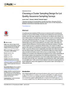
Fig. 1. Diagrammatic representation of cluster sampling protocol used in broccoli Þelds.
marked in a Þeld according to a standard V-shaped pattern that extended from one corner of the Þeld, to the midpoint on the other side, and back to the adjacent corner (Hoy et al. 1983, Torres and Hoy 2002). Along each transect, there were Þve equidistantly spaced sampling points. At each point, the total number of larvae (all instars) on four nearby plants (elements) was recorded. Each of these groups of four plants formed a cluster, and there were 10 clusters, resulting in 40 elements in total. All crops were planted in beds that consisted of two staggered rows of plants. The four plants chosen for sampling were from the bed nearest to the sampling point. From this bed, the nearest two plants in the row closest to the sampling point were sampled as well as the two closest plants in the next row. Thus, at each cluster, equal numbers of elements from both sides of the bed were sampled. Surveys were conducted on properties in the Cranbourne and Werribee vegetable growing regions on MelbourneÕs outer eastern and western fringes, respectively. In total, 23 crops were surveyed from the Werribee region and seven from around Cranbourne. Each crop was surveyed at approximately weekly intervals from 1 wk after transplant through to harvest (usually ⬇7 to 8 wk). Growers maintained normal spray practices (typically calendar spraying) throughout the period of data collection. Variance Estimation and Regression for Taylor’s a and b Parameters. The simplest way to estimate the variance among all elements in the population (2) would have been to use the variance associated with the 40 elements in the sample. This unadjusted sample variance (s2) is, however, a slightly biased estimate of 2, because the elements were drawn from contiguous groups (i.e., clusters) rather than at random. We used the method of Cochran (1977, p. 239) to obtain an (almost) unbiased variance estimate, s 2u . However, for our data set this adjustment led to negligible changes
1133
in the estimates of TaylorÕs a and b parameters (⬍1.2 and ⬍0.09%, respectively). TaylorÕs a and b parameters were estimated by regressing ln s 2u against ln xˆ . Because there was error associated with estimating both s 2u and x , BartlettÕs regression method was used (Bartlett 1949). The regression was done using a BASIC program (Legg 1986), and the data were sorted according to the independent variable. To make inferences about the spatial distribution of the species, we tested the null hypothesis that the slope was not signiÞcantly different from one by using the t-test procedure of Bartlett (1949). There was one singleton observation (i.e., an observation where larvae were only observed in one element), and this was excluded from all analyses, because the values of s2 and x are restricted for singleton observations (s2 ⫽ x ), which leads to pseudorandomness (Taylor 1984). Sample Size Adjustment. The regression parameters obtained from a TPL plot based on the s 2u estimates could be used to develop a sequential sampling plan using GreenÕs (1970) method. However, such a plan assumes that SRS (or at least SRegS) would be used, and this is clearly not going to be so for plans that include clusters of elements (i.e., like the sampling procedure described above that was used to collect the data for this study). A plan based on these TaylorÕs a and b values would give an underestimate of the minimum sample size. Consequently, the stop-lines for the sequential plan would also be incorrect. We adjusted for this by using the design effect (deff) (Kish 1995, pp. 162 and 257). The deff is the ratio of the variance obtained from a complex sample to the variance obtained from a SRS of the same number of units (or elements). For the cluster sampling used in the broccoli Þelds, deff ⫽ MSc2/s 2u
[3]
This formula for the deff is sometimes written with a factor, 1 ⫺ f, in the denominator, where f is the sampling fraction (sample size/population size). However, in this study, and those to which the results will be applied, f is negligible, and so the factor (being close to 1) can be omitted. Note that the deff formula as deÞned by Kish (1995, pp. 162 and 257) uses the actual between cluster variance rather than MSc2 . Although the MSc2 is not a readily interpretable quantity, unlike the between cluster variance, it makes the computation of the deff more simple, because it can readily be calculated using nested analysis of variance (ANOVA). In this way, the deff can be calculated separately for each observation. However, it is likely to vary substantially across observations, and in most cases we want to calculate an overall deff, for use in future sampling plans. Thus, it is necessary to perform a nested ANOVA covering all observations to calculate MSc2 and s 2u . If the data are unbalanced (e.g., variable numbers of elements per cluster across sampling occasions), then a restricted maximum likelihood analysis should be used in preference to ANOVA (Patter-
1134
JOURNAL OF ECONOMIC ENTOMOLOGY
Vol. 97, no. 3
TPL described the variance-mean relation well (r2 ⫽ 0.90) (Fig. 2). The slope of the Þtted line, 1.39, was signiÞcantly greater than unity (t ⫽ 3.42, df ⫽ 23, P ⬍ 0.01), indicating that overall the “population” had a contagious distribution. This is consistent with observations of the spatial distribution of P. xylostella on other Brassica vegetable crops. On caulißower, P. xylostella larvae (data pooled across all instars) demonstrated a contagious distribution, with slopes of 1.41 and 1.31 for TPL and IwaoÕs (1968) mean crowding on mean density plots, respectively (Chen and Su 1986). In a study of P. xylostella larvae in a commercial cabbage crop, TPL gradients of 1.35 and 1.26 were re-
ported for data sets collected by two different scouts (Trumble et al. 1989). Sivapragasam et al. (1986) described a contagious distribution for P. xylostella eggs, larvae (all instars pooled) and pupae on cabbages using IwaoÕs (1968) plots. Fitting of the negative binomial distribution has also been used to demonstrate departures from the Poisson distribution, and the exponent k can be used as a measure of contagion. Harcourt (1960) Þtted the negative binomial distribution to eggs, each instar and pupae on cabbage. For all of these life stages, k remained reasonably stable with changes in density and suggested a contagious distribution. However, when considering all instars together on caulißower, Chen and Su (1986) could not detect a constant k across different densities. The contagious distribution of larvae observed in the current study is probably a function of the tendency of females to lay groups of eggs on the one plant. Although some dispersal of early instars, driven by crowding, and of mature larvae looking for pupation sites, is likely to occur (Harcourt 1960), this does not seem to be sufÞcient to lead to a noncontagious larval distribution. The overall deff in this example was 1.31. The fact that the deff was ⬎1 meant that more samples would need to be collected to satisfy the stop rule in the deff-corrected plan as opposed to the uncorrected plan (Figs. 3 and 4). The disparity between the two plans increased as the nominal level of precision increased (i.e., as D decreased). Precision levels of around 0.2 or 0.3 would be considered practicable for pest sampling (Southwood 1978), whereas higher precision, e.g., D ⫽ 0.1, is usually desired for research purposes (Manly 1989). Thus, the unadjusted sampling plan would underestimate the number of samples that would need to be collected to achieve the desired level of precision. This is particularly so at mean densities of about 0.5 to 1 larvae per plant (Fig. 2), and such densities are not uncommon in sprayed crops in practice (Fig. 2). In general, the sample sizes demanded by the D ⫽ 0.1 and 0.2 sampling plans (Fig. 2) would be considered practicable, but this would not be so for the D ⫽ 0.1 plan. Thus, in Australia and New
Fig. 2. TaylorÕs power plot for diamondback moth in broccoli. ln s2 ⫽ 0.63 ⫹ 1.39 ln x , r2 ⫽ 0.90.
Fig. 3. Minimum sample sizes for three levels of precision. Solid lines indicate that the sample size has been adjusted using the deff, whereas dashed lines are unadjusted.
son and Thompson 1971, Hepworth and Hamilton 2001). Sampling Plan Construction. The minimum sample size (nmin) for GreenÕs (1970) plan was calculated as follows: nmin ⫽ s2u/共Dx 兲2 where D is the nominal desired level of precision, expressed in terms of the standard error as a fraction of the mean. The sequential sampling stop-line (Tn) was calculated as follows: Tn ⫽
冉冊 D2 aˆ
ˆ 1/共b-2兲
ˆ
ˆ
nmin 共b⫺1兲/共b⫺2兲
where aˆ and bˆ are the TPL regression parameters, estimated as described above. A sequential sampling chart is usually constructed by plotting Tn against nmin (Green 1970). However, here we needed to multiply nmin by the deff to correct for the fact that sampling with clusters of four plants will be used for monitoring the crop. Thus, Tn was plotted against an adjusted minimum sample size (nminA ⫽ nmin.deff). Note that the calculation of Tn is based on nmin not nminA. If nminA was used in the calculation of Tn, and also in the plot, the inßuence of the deff would cancel itself out. Results and Discussion
June 2004
HAMILTON AND HEPWORTH: ACCOUNTING FOR CLUSTER SAMPLING
1135
and a larger number of elements per cluster results in a variance that is much greater.
Acknowledgments This work was funded by the AusVeg Levy and Horticulture Australia. We are grateful to Nancy Endersby and others who scouted the crops and to several growers for allowing us to sample properties. Peter Ridland provided useful comments on a draft of the manuscript.
References Cited Fig. 4. Critical stop-lines for three levels of precision. Solid and dashed lines as for Fig. 2. Note the different tick intervals for the upper and lower portions of the y-axis.
Zealand, where P. xylostella is typically the only major lepidopteran pest, this plan could provide a useful alternative to the binomial plans of Hamilton et al. (2004) and Mo et al. (2004). The deff has been used here to adjust the minimum sample size for GreenÕs (1970) sequential plan, but it can be applied to any type of sequential sampling plan. For example, it could also be used to adjust the minimum sample size for KunoÕs (1969) plan, which is the other most commonly used enumerative sequential plan. The deff has also been used to adjust the variance estimate used in a presence-absence sampling plan and was found to have a particularly marked inßuence when a small proportion of the sampling units was infested (Hepworth and McFarlane 1992). The deff was used here to adjust for a two-stage design, but it could also be used to correct for multistage designs. Furthermore, it is appropriate for hierarchical designs other than clustering, such as stratiÞed sampling. However, whereas the deff would usually be expected to be ⬎1 for cluster sampling, it would typically be ⬍1 for stratiÞed samples (Kish 1995, p. 259). The deff is ⬎1 for most cluster samples because the elements within the clusters are often correlated. In contrast, the very purpose of stratiÞed sampling is usually to reduce the overall variance associated with the estimate of the mean. Thus, the variance estimate obtained from a stratiÞed sample would be expected to be less than that from a SRS of the same number of units or elements, which would lead to a deff of ⬍1. The deff could also be used to adjust for a design similar to that used in this study, but with the number of elements per cluster (d) being different from four (the number used here). The numerator in equation 1 can be expressed as MSc2 ⫽ ds c2 ⫹ MSc2 where s c2 is the between cluster variance, which is easily calculated from the ANOVA. Substituting a different number for d results in a deff different from 1.31. For example, d ⫽ 2 results in deff ⫽ 1.10, and d ⫽ 8 results in deff ⫽ 1.72. As expected, a smaller number of elements per cluster results in a variance more similar to that of a SRS with the same total number of elements,
Allsopp, P. G., T. L. Ladd, Jr., and M. G. Klein. 1992. Sample sizes and distributions of Japanese beetles (Coleoptera: Scarabaeidae): captured in lure traps. J. Econ. Entomol. 85: 1797Ð1801. Bartlett, M. S. 1949. Fitting a straight line when both variables are subject to error. Biometrics 5: 207Ð212. Binns, M. R., J. P. Nyrop, and W. van der Werf. 2000. Sampling and monitoring in crop protection: the theoretical basis for developing practical decision guides. CABI Publishing, New York Chen, C., and W. Su. 1986. Spatial pattern and transformation of Þeld counts of Plutella xylostella (L.) larvae on caulißower. Plant Protect. Bull. (Taiwan, R.O.C.) 28: 323Ð 333. Cho, K., C. S. Eckel, J. F. Walgenbach, and G. G. Kennedy. 1995. Spatial distribution and sampling procedures for Frankliniella spp. (Thysanoptera: Thripidae) in staked tomato. J. Econ. Entomol. 88: 1658 Ð1665. Cochran, W. G. 1977. Sampling techniques. Wiley, New York. Green, R. H. 1970. On Þxed precision level sequential sampling. Res. Popul. Ecol. 12: 249 Ð251. Hamilton, A. J., N. Schellhorn, N. E. Endersby, P. M. Ridland, and S. A. Ward. 2004. A dynamic binomial sequential sampling plan for Plutella xylostella (Lepidoptera: Plutellidae) on broccoli and caulißower in Australia. J. Econ. Entomol. 97: 127Ð135. Harcourt, D. G. 1960. Distribution of the immature stages of the diamondback moth, Plutella maculipennis (Curt.) (Lepidoptera: Plutellidae), on cabbage. Can. Entomol. 92: 517Ð521. Hepworth, G., and A. J. Hamilton. 2001. Scan sampling and waterfowl activity budget studies: design and analysis considerations. Behavior 138: 1391Ð1405. Hepworth, G., and J. R. McFarlane. 1992. Variance of the estimated population density from a presence-absence threshold sample. J. Econ. Entomol. 85: 2240 Ð2245. Hoy, C. W., C. Jennison, A. M. Shelton, and J. T. Andaloro. 1983. Variable-intensity sampling: a new technique for decision making in cabbage pest management. J. Econ. Entomol. 76: 139 Ð143. Hutchison, W. D. 1994. Sequential sampling to determine population density, pp. 207Ð244. In L. P. Pedigo and G. D. Buntin [eds.], Handbook of sampling methods for arthropods in agriculture. CRC, Boca Raton, FL. Iwao, S. 1968. A new regression method for analyzing the aggregation pattern of animal populations. Res. Popul. Ecol. 10: 1Ð20. Kish, L. K. 1995. Survey sampling. Wiley, New York. Kuno, E. 1969. A new method of sequential sampling to obtain population estimates with a Þxed level of precision. Res. Popul. Ecol. 11: 127Ð136.
1136
JOURNAL OF ECONOMIC ENTOMOLOGY
Legg, D. E. 1986. An interactive computer program for calculating BartlettÕs regression method. North Central Computer Inst. Software J. 2: 1Ð23. Manly, B. F. 1989. A review of methods for the analysis of stage-frequency data, pp. 3Ð 69. In L. McDonald, B. Manly, J. Lockwood, and J. Logan [eds.], Estimation and analysis of insect populations. Springer, Berlin, Germany. Mo, J., G. Baker, and M. Keller. 2004 Evaluation of sequential binomial sampling plans for decision-making in the management of diamondback moth (Plutella xylostella) (Plutellidae: Lepidoptera). In Proceedings of the 4th International Workshop on the Management of Diamondback Moth and other Crucifer Pests, 15Ð26 November 2001, Melbourne, Australia. Department of Natural Resources and Environment, Melbourne, Australia. Patterson, H. D., and R. Thompson. 1971. Recovery of interblock information when block sizes are unequal. Biometrika 58: 545Ð554. Sivapragasam, A., Y. Ito, and T. Saito. 1986. Distribution patterns of immatures of the diamondback moth, Plutella xylostella (L.) (Lepidoptera: Yponomeutidae) and its lar-
Vol. 97, no. 3
val parasitoid on cabbages. Appl. Entomol. Zool. 21: 546 Ð 552. Smith, A. M., and G. Hepworth. 1992. Sampling statistics and a sampling plan for eggs of pea weevil (Coleoptera: Bruchidae). J. Econ. Entomol. 85: 1791Ð1796. Southwood, T.R.E. 1978. Ecological methods: with particular reference to the study of insect populations. Chapman & Hall, London, England. Taylor, L. R. 1961. Aggregation, variance and the mean. Nature (Lond.) 189: 732Ð735. Taylor, L. R. 1984. Assessing and interpreting the spatial distributions of insect populations. Annu. Rev. Entomol. 29: 321Ð357. Torres, A. N., and C. W. Hoy. 2002. Sampling scheme for carrot weevil (Coleoptera: Curculionidae) in parsley. J. Econ. Entomol. 31: 1251Ð1258. Trumble, R. H., M. J. Brewer, A. M. Shelton, and J. P. Nyrop. 1989. Transportability of Þxed-precision level sampling plans. Res. Popul. Ecol. 31: 325Ð342. Received 23 June 2003; accepted 22 January 2004.