A SHAPE-BASED FINITE IMPULSE RESPONSE MODEL FOR FUNCTIONAL BRAIN IMAGES Bing Bai
Paul Kantor
[email protected] Department of Computer Science Rutgers University
[email protected] Department of Computer Science Rutgers University
ABSTRACT We present a new Finite Impulse Response (FIR) model for hemodynamics in functional brain images. Like other FIR models, our method permits a flexible formulation of the hemodynamic response. The distinctive feature of this model is that the shape information of the canonical HRF is imposed on the FIR, with little loss of flexibility. Model fitting involves minimizing quadratic error under linear constraints. Our model proves more robust to noise on both synthetic data and real data, in contrast to other FIR models. Index Terms— functional magnetic resonance imaging, fMRI, finite impulse response, hemodynamic response, HRF
falls back to “idle” mode (with an apparent undershoot) gradually after that. The canonical HRF shown is generated as the difference of two gamma probability density functions: 1 H(t) = f (t; 6, 1) − f (t; 16, 1), 6
1 tα−1 e−t/β for t > 0. This model where f (t; α, β) = β α Γ(α) is often referred to as the “double gamma function”. The first term controls the major shape of the “hill”, while the second one is responsible for the undershoot. Figure 1(b), a “single gamma function”, is a simplified version with the second gamma function removed. (a) Double gamma function
1. INTRODUCTION fMRI (functional Magnetic Resonance Imaging) [1] is an imaging technique used to “monitor” brain activities. The most widely used fMRI method is BOLD (blood oxygen level dependent) fMRI, where the intensity of an image element (it is called a voxel in 3D images, corresponding to a “pixel” for 2D images) is related to the level of blood oxygen in the corresponding region. When a cognitive process involves a specific brain region, at first, oxygen is consumed, but more oxygen is brought in by blood flow soon after, and this change will brighten the brain region in the image. The most widely used mathematical method for fMRI research is the general linear model (GLM) [2, 3], in which the time series of signal intensity at each voxel is modeled as a linear combination of explanatory variables and Gaussian noise. An explanatory variable (EV) arises from the hypothesized response to a certain type of stimulus. More specifically, the time dependent EV is generated by convolving the stimulus time series with a impulse response function, which is called the hemodynamic response function (HRF). The nature of the HRF has been extensively studied [1]. A widely used assumption for the HRF is that its shape should be somewhat as in Figure 1(a), which is called the “canonical HRF” [1]. Specifically, when a cognitive event occurs, initial consumption of oxygen causes a small dip. The level of refreshing blood oxygen reaches a peak in about 4-6 seconds, and then
(1)
(b) Single gamma function
0.2
0.2
0.15
0.15
0.1
0.1
0.05
0.05
0
0
−0.05
−0.05
0
10
20
30
0
10
20
30
Fig. 1. Canonical Hemodynamic Response Function. While the canonical HRF works very well in many experiments, it is believed that the real HRF varies in different people, and in different brain regions of the same person [1]. More flexible models, such as the Finite Impulse Response (FIR), have been proposed [4]. In this model, the activation of a certain voxel at time t is the weighted sum of the stimuli (si , i ∈ [t−n+1, t]) at the preceding n time points. Formally, yt =
n X
wi st−(i−1) + w0 + ǫ,
(2)
i=1
where yt is the intensity value at time t, ǫ is guassian noise, and w0 is the constant component. The optimal estimate of w = [w0 , w1 , w2 , ...wn ]T is defined as the one that minimizes the squared error between the observation and the model: wopt = argmin w
N X t=n
(yt − yˆt (w))2 ,
(3)
where yˆt (w) =
n X
some delay, p, so that wi st−(i−1) + w0 ,
(4)
wi−1 ≤ wi wi ≥ wi+1
i=1
and N is the length of observation/stimuli sequence. This is a linear regression problem. Written in matrix form, Eq. (2) becomes: Sw = y + ǫ, where 1 sn sn−1 ... s1 1 sn+1 sn ... s2 , S= 1 ... ... ... ... 1 sN sN −1 ... sN −n+1 w = [w0 , w1 , w2 , ..., wn ]T , and y = [yn , yn+2 , ..., yN ]T , and the optimal estimate of w is w = [ST S]−1 ST y. Compared to the canonical HRF, whose shape is basically fixed, this “naive” FIR model is very flexible, and thus has the potential to describe a greater variety of hemodynamic behaviors. However, this model tends to overfit as the number of parameters increases, especially under considerable noise, which is exactly the case for fMRI images. A typical observation is that large positive and large negative weights may appear alternately, as we will show in section 3. To overcome this problem, Goutte et al. [4] use a maximum a posteriori (MAP) parameter estimation similar to ridge regression: wMAP = (ST S + varΣ−1 )−1 ST y,
(5)
where Σij = v exp(− h2 (i − j)2 ), in which h is a smooth factor, v is the strength, var is the variance of noise (in [4] it is referred to as “σ 2 ”, we rename it to avoid notational conflict). The correlation among parameters prevents sudden changes (spikes) in the form of the HRF. Although the “smoothing” in this Bayesian FIR model can eliminate high frequency noise to some degree, it has the following limitations: First, it requires careful selection of the hyper parameters, h, v and var. Second, and more important, although MAP estimation can smooth changes between neighboring parameters, our experiments show that it can not remove large negative values and multiple peaks without making the whole HRF too flat. We propose to address these problems by injecting prior knowledge about the canonical HRF into FIR models, without much loss of flexibility. Specifically, we impose shape information derived from the single gamma HRF on the FIR model, as linear constraints. Thus, the linear/bayesian regresssion problem becomes a constrained optimization problem. We show that, with both synthetic data and real data, this new method we propose (SPNN: Single Peak Non-Negative FIR), effectively controls the drawbacks of the MAP model. 2. THE SINGLE PEAK NON-NEGATIVE (SPNN) FIR MODEL We propose an FIR model with the objective function (3), together with following constraints: 1) there is a single peak at
: i ∈ [2, p] : i ∈ [p, n − 1]
(6)
2) all weights are non-negative: wi ≥ 0, i ∈ [1, n]
(7)
These two sets of constraints help us to keep the major shape feature of the canonical HRF: 1) the majority of responses stay positive; 2) the response rises to a single maximum and decays after that. Note that the initial dip and the recovery undershoot are lost in this model. For each value of the location of peak p, the problem is then to minimize the objective function of (3) subject to the constraints (6) and (7). This is a quadratic programming problem. If we write the objective as follows: N X
(yt − yˆt (w))2 =
t=n
N X
yt 2 −
t=n
N X t=n
2yt yˆt (w) +
N X
yˆt (w)2 ,
t=n
we notice that the third term yˆt (w)2 contains all the quadratic terms and only the quadratic terms in the weights wi , i ∈ [0, n], and it is always non-negative. This means that the problem is a semi-definite quadratic programming problem and a global optimal solution can be found via a variety of methods such as the interior-point method and the active set method [5]. So far, we have assumed that the peak location p is given. In fact, to determine the location of the peak, we repeat the above procedure for each p ∈ [1, n], and then retain the weights which generates the minimum. SPNN and MAP are two different approaches to dealing with the overfitting problem (SPNN uses shape information while MAP uses parameter correlation). It is natural to suggest mixing the two. Indeed, SPNN can be easily combined with the smoothing idea in Goutte et. al [4]. To do this, we note that the MAP estimate (5) minimizes the following objective with no constraints: P
min
N X
(yt − yˆt (w))2 + wT Σ−1 w.
(8)
t=1
The constant w0 should not be penalized, thus the element (1,1) should be reset to 0 for Σ−1 . By imposing the linear constraints of (6) and (7) on the objective (8), we obtain a quadratic programming problem, whose solution may combine merits of SPNN and MAP estimation. 3. RESULTS ON SYNTHETIC DATA In this section, we first generate a synthetic brain response by convoluting a hypothesized HRF with a hypothesized stimulus. A good model should recover the HRF from this synthetic
(a) Linear Regression
(b) MAP
(c) SPNN
(d) SPNN−MAP
(e) Simple NN
0.4
0.4
0.4
0.4
0.4
0.2
0.2
0.2
0.2
0.2
0
0
0
0
0
−0.2
−0.2
−0.2
−0.2
−0.2
0
4
8 12 16 20 24 28 Seconds
0
4
8 12 16 20 24 28 Seconds
0
4
8 12 16 20 24 28 Seconds
0
4
8 12 16 20 24 28 Seconds
0
4
8 12 16 20 24 28 Seconds
Fig. 4. Box plot for weight estimation for 100 repeated experiments (a) Canonical HRF (TR=2)
(b) Stimuli and Synthetic Response
0.2
1.5 Stimuli Syn Resp
0.15 1 0.1 0.5 0.05 0
0 0
5
10 Seconds
15
20
0
10
20
30
40
50 60 Seconds
70
80
90
100
Fig. 2. Synthetic data HRF Weights estimate for noise level 1.5 0.4 0.3 lr map
0.2
spnn spnn−map
0.1 0 −0.1 −0.2
0
5
10
15 Seconds
20
25
30
Fig. 3. Recovered weights from synthetic data
response, under a reasonable amount of noise. We select the HRF as a single gamma function with the sampling period (corresponding to TR) set to 2 seconds (shown in Figure 2 (a)), because it is a typical setting in many fMRI experiments. We take the time range from 0 to 20 seconds, 11 weights in all (not including the constant w0 ). The stimulus is a random binary sequence of length 100, with equal probabilities for “0” and “1”. They are shown together with generated synthetic response in Figure 2(b). We then add noise to this explanatory variable to simulate an “observation” time series. The noise ∈ N (0, σ 2 ). we call σ 2 the Noise Level. When the noise level is set to 0, all methods give very good estimates. In the rest of this paper, we set the noise level to 1.5, which is fairly large comparing to the synthetic response in Figure 2. We compare the recovered HRF from linear regression (LR), MAP, SPNN and MAP combined with SPNN constraints (SPNN-MAP). We set the hyper parameters of MAP to h = .3, v = .1, var = 1. Note that we are not trying to find optimal values for these parameters, the choice of these hyper
parameters will not affect our conclusion, as long as the same values are used in all experiments. In Figure 3, to test the robustness of the methods when the width of the HRF is unknown, we set n = 15 instead of the real length of the HRF n = 11. We see that pure linear regression (LR) is seriously overfitting, with many changes of sign. Although MAP gives a smooth curve by filtering out high frequency noise, and reduces the error in parameter estimation, it still produces a large negative dip, and a heavy bump at late times. SPNN and SPNN-MAP both achieve good performance, but the curves of SPNN-MAP are more smooth. We repeat the experiments 100 times, with random noise generated with the same noise level of 1.5. We show boxplots [7] for each method in Figure 4. The bottom of a box is the value of the first quartile, the top is that of the third quartile, while the bar in the middle is the median. There are also two “nails” (called “whiskers”) that stick out upward and downward. They indicate the maximum and minimum values, or 1.5 times the height of the box (which is called inter-quartile range (IQR)) from the median, which ever is closer to the median. For the latter case, all values outside that range of whiskers are considered “outliers” (shown as dots). We see the medians in all 4 plots match very well to the true HRF, which is marked with small circles. Due to the smoothing factor, the estimated curves for MAP and SPNN-MAP are flattened a small amount. Linear regression apparently has largest variance in parameter estimation. MAP effectively reduces this variance. However, MAP shares the defect of linear regression that the variance does not diminish as the lag increases, and that is the cause of the oscillation in Figure 3. On the other hand, the estimates of SPNN decrease for larger lag, but it has a relatively large number of outliers. Also in Figure 3, the SPNN-MAP method combines the advantages of both SPNN and MAP. We still see a number of outliers in the figure for SPNN-MAP, but note they are actually below the upper whiskers of MAP estimations. SPNNMAP makes the boxes quite small, and points are more likely to be considered as “outliers”. Simple NN (non-negativity) serves as a null model. It is the same as MAP except all the negative values are set to 0. we see the variation does not decrease at late times as much as for SPNN and SPNN-MAP. This method is included to show the performance gain produced by SPNN is not trivial.
Linear Regression
SPNN
MAP
15
15
10
5
10
10
5
5 0
5
5
0
−5
0 0
4
8 12 16 20 24 28 Seconds
Simple NN
SPNN−MAP 10
10
15
0
4
8 12 16 20 24 28 Seconds
0 0
4
8 12 16 20 24 28 Seconds
0 0
4
8 12 16 20 24 28 Seconds
0
4
8 12 16 20 24 28 Seconds
(a) Oddball auditory, 4 datasets, 20 voxels Linear Regression
MAP
SPNN
0
10
6
5
5
Simple NN
SPNN−MAP 8
10
10
4
5
0
5
2 −5
−5 0 3 6 9 12 15 18 21 24 Seconds
0 0 3 6 9 12 15 18 21 24 Seconds
0 0 3 6 9 12 15 18 21 24 Seconds
0 0 3 6 9 12 15 18 21 24 Seconds
0 3 6 9 12 15 18 21 24 Seconds
(b) Event perception [6], 25 datasets, 125 voxels Fig. 5. Parameter estimation for real fMRI datasets 4. MODEL FITTING: RESULTS ON REAL DATA Due to page limits, we show experimental results from a few experiments in depth, but the results in other datasets are quite similar. In Figure 5, we compare the 4 methods on the following experiments. 1) Oddball auditory: subjects are presented with unexpected sound. 2) Event perception [6]: subjects watching cartoon objects. The MAP hyper parameters are still h = .3, v = .1, var = 1. The length of FIR is set to be less than 30 seconds, which is usually considered long enough for hemodynamic responses. We select as the top 5 voxels from each dataset that have the largest t-values in GLM analysis with double gamma function. This is to avoid selecting inactive voxels. As we observed for synthetic data, the SPNN method reduces the variance in HRF tail, while MAP reduces the variance overall. Their combination gives the most robust parameter estimation. 5. DISCUSSIONS AND CONCLUDING REMARKS The move from phantom data to real data has provided some expected confirmations, and some puzzling new phenomena. As expected, the SPNN-MAP performs quite well, producing smooth parameter estimates, with relatively tight variation, and with very few “late lag” artifacts. On the other hand, the precise location of the peak in all of the models is surprising. Assuming that we can read the “typical shape” of a solution by the shape of the median points, we see that all methods, whether or not they are constrained to yield positive weights, seem to peak considerably later than the very model that was used in the analysis of the data (recall that we selected these voxels by GLM based on double gamma function). There are several possible explanations, which invite further study. One possibility is that the selected voxels (which are in real
brains) may have a response which matches “well enough” to the double gamma function, but is even more accurately described ’by a single peak which occurs somewhat later than is usually believed. While these questions remain open, the results shown here indicate that with modern computation methods the apparent complexities of quadratic programming can be surmounted, and that the extensions to the FIR approach show promise in the robust analysis of realistic and noisy data. 6. ACKNOWLEDGEMENT This work is supported by NSF grant ITR-0205178. We thank Nicu Cornea, Sven Dickinson, Ali Shokoufandeh and Deborah Silver for their helpful advice and encouragement. We particularly thank Co-PI Stephen Hanson for providing the fMRI datasets used in this analysis. 7. REFERENCES [1] R.S.J. Frackowiak, K.J. Friston, C.D. Frith, R.J. Dolan, C.J. Price, S. Zeki, J. Ashburner, and W. Penny, Human Brain Function (2nd Edition). [2] K.J. Friston, P. Jezzard, and R. Turner, “Analysis of functional MRI time-series,” Human Brain Mapping, vol. 1, pp. 153–171, 1994. [3] J. Fox, Linear statistical models and related methods, 1984. ˚ [4] Cyril Goutte, Finn Arup Nielsen, and Lars Kai Hansen, “Modelling the haemodynamic response in fmri with smooth fir filters.,” IEEE Trans. Med. Imaging, vol. 19, no. 12, pp. 1188–1201, 2000. [5] J. Nocedal and S. Wright, Numerical Optimization, Springer, 1999. [6] A. Zaimi, C. Hanson, and S.J. Hanson, “Event perception of schemarich and schema-poor video sequences during fmri scanning: Top down versus bottom up processing,” in In Proceedings of the Annual Meeting of the Cognitive Neuroscience Society, 2004. [7] J.W. Tukey, Exploratory Data Analysis, Addison-Wesley, 1977.