A Signal Aware Movement Control Algorithm for GPS-free Ad Hoc Networks Ying Zhang, Zhong Shen, Yilin Chang Zhongjiang Yan, Liang Dai
A Signal Aware Movement Control Algorithm for GPS-free Ad Hoc Networks Ying Zhang, Zhong Shen, Yilin Chang Zhongjiang Yan, Liang Dai State Key Laboratory of ISN, Xidian University, Xi’an 710071, PR China,
[email protected] doi:10.4156/jcit.vol5. issue9.25
Abstract A movement control algorithm is presented to improve the performance of mobile Ad Hoc networks on condition that positions are unavailable for nodes. The algorithm proposes a way to move the mobile nodes to the optimal position, only according to the detected signal strength. Beginning with the definition of the performance function, the article then proves that the moving target can be fixed at the point with the optimal solution of the function. The algorithm leads the mobile node into the optimal location from anywhere it stays. Finally, the simulation results show that the newly designed movement algorithm can be used to seek out the optimal point, and meanwhile minimize the transmission cost by moving the node to this point.
Keywords: Movement Control, Signal Strength, GPS-free Ad Hoc Network, Optimal Searching 1. Introduction In the past, many works studied on the mobile Ad Hoc networks often considered the node mobility as a negative factor which causes link break, disconnections and so forth. In recent years, it has been proposed that the mobility can be potentially used to improve network performance [1], especially for the case that affected by such factors as environment, energy and etc., link quality cannot meet the communication requirement even with the maximum transmission power. Taking into account the fact that most of the mobile hosts are characterized by battery-equipped devices, and conserving energy is a key factor for the Ad Hoc networks, thus controlled mobility for energy conservation is motivated. The controlled mobility can be defined as a kind of movement which mobile nodes move to some specified destinations for specific objectives. The application of movement control as a new method to improve the performance of Ad Hoc networks represents a new direction of the topology management. In fact, the use of controlled mobility still needs to be explored in depth. For example, some controlled mobility algorithms have been proposed in [2-7]. However, to the best of our knowledge, they are unsuitable for GPS-free Ad Hoc networks. In this paper, we propose a movement control algorithm for Ad Hoc networks, where all the nodes are not equipped with GPS and other localization method. The idea is to move nodes to the favorable location by investigating the detected signal strength to achieve further improvements in terms of network performance as connectivity and energy consumption. The rest of the paper is organized as follows. Section 2 is the related works. Both the optimal location of the mobile node and details about the movement control algorithm are described in Section 3. Section 4 is related to simulation, and finally we conclude our work in Section 5.
2. Related Work In practice, the movement control scheme can be effectively used to enhance the network performance by allowing mobile nodes to reach favorable positions. Basu et al [2] presented a centralized movement control algorithm. However, it is unsuitable for large scale network, because every node should acquire global information of the network. Being aware of the problem, S. Das et al [3][6] proposed a distributed algorithm. Communication links are established to form a survivable network topology by moving some nodes together. Although the algorithm shows efficiency for gathering the information and the updated network configuration dose improve the robust of the network, the optimal locations of mobile nodes have not yet clearly defined. Another mobility control scheme [4] pointed out that the movable node must lie in the middle of its two successive
238
Journal of Convergence Information Technology Volume 5, Number 9. November 2010
communication neighbors, so as to improve the energy efficiency as well as the network connectivity. Based on [4], Z. Jiang et al [5] proposed a similar scheme to control the movement with the node’s phop neighborhood. Simulations show that oscillation can be avoided which is valid in convergence. X. Chen et al [7] also use the optimal location information of the mobile node as a guide speed up the convergence process while minimizing the transmitting cost. Though nodes redeployment, other schemes aim to maximize the node coverage and even construct a long -lived network [8][9]. Generally, these existing movement control algorithms are readily implemented on the assumption that positions are known for each node. However, mobile nodes, in many practical applications, are not equipped with GPS or other localization method. So it will be hard for them to find out the optimal points instantly due to no available information of the positions. Accordingly, a new designed movement control algorithm based on the analytical results obtained in [4][5][7] is presented, leading the mobile node into the middle of its neighbors, which should be the optimal position for the mobile node. Here, nodes move without the position information but the receiving signal strength (RSS). When operated iteratively with detecting RSS, moving is adjusted so as to improve the link effectiveness and minimize the transmitting consumption.
3. The signal aware movement control algorithm (SAMC) 3.1. Network model We assume that all the nodes have the same transmission range. Two nodes within each other's transmission range are neighbors and can be communicate directly to each other. Otherwise they have to rely on intermediate nodes to relay the messages for them. As seen in figure 1, data transmitted between node A and node B involves node C. Assuming that node A and B are stationary, communications between A and B can be further improved by relocating node C to optimal position. In [1], D. Goldenberg et al have illustrated that the transmitting cost from A to B can be minimized when C moves to Copt, the midpoint of the line segment AB, so the position of Copt xCopt can be represented as
1 xCopt ( x A xB ) , 2
(1)
where xA , xB are positions of A and B. Copt O
B
A
C
Figure 1. Optimal position of node C More generally, node C always keeps in touch with more than two neighbors, so a constraint on the motion of node C is imposed by its other neighbors. In this situation, Copt is altered to the point which is closest to the midpoint of AB. When mobile nodes are not equipped with GPS or other localization method, nodes can move without the position information but the RSS. Next, we will introduce wherever the Copt actually locates.
3.2. The optimal position
239
A Signal Aware Movement Control Algorithm for GPS-free Ad Hoc Networks Ying Zhang, Zhong Shen, Yilin Chang Zhongjiang Yan, Liang Dai
While Copt seems unachievable for nodes do not equip with GPS or other localization methods. We still expect that Copt can be reached although positions are unobtainable for node C. Fortunately; we can lay our hope on RSS, the only information received from the neighbor nodes. A performance function of the signal strength when node C stays at any position x is defined as
( x) Ri 1( x) ,
(2)
iSn
where R is signal strength, Sn is the neighbor set of C. 2 Taking into account the theory that transmitting power should be attenuated in accordance with d , where d is the distance between the transmitter and the receiver. So the received signal can be noted as 2 t t Gr , where Gt, Gr are R=kd-2, on condition that the transmitted power Pt is given. Here k PG 2 4 antenna gains of the transmitter and the receiver respectively, and cf is the wavelength. Thus, Eq.(2) can be rewritten as 2 ( x ) k -1 ( x xi ) .
(3)
iSn
The gradient of x, denoted asx, is given by differentiating Eq.(3) with respected to x, ( x )
1 2k x xi x iSn
T
2k 1 y yi , iSn
(4)
Where (x,y) and (xi, yi) are positions of the mobile node and its neighbors. Then x is set to its optimal value xCopt when x=0 and x n (n is the total number of its neighbors).
iS n
xCopt
xi iSn n
yi iS n
n
T
.
(5)
Obviously, xCopt is the gravity center of the convex polygon composed by neighbors. Specifically, for n=2, which is the case showed in figure 1, xCopt is the midpoint of the line segment composed by the two neighbors A and B. Then differentiating twice, we have that 2nk 1 0 . 2 ( x ) 0 2nk 1
(6)
For k>0 and n>0, 2x is a positive-definite matrix. So we believe that xCopt is the optimal solution of x, and xCopt) is the minimum of x A portion of a typical x is illustrated in figure 2. The vertical axis represents the value of x and the horizontal axes the position of the mobile node. The bowl-shaped x is a paraboloid with the concave surface upward. Contours of constant x are elliptical, as can be seen by setting x constant in Eq.(3). The point at the bottom is projected onto the horizontal plane as xCopt, corresponding with the minimum of x. Therefore, the procedure that causes node C to locate xCopt can be regarded as xCopt arg min ( x), x R .
240
(7)
Journal of Convergence Information Technology Volume 5, Number 9. November 2010
xCopt y position x position
Figure 2. Portion of x
3.3. The SAMC algorithm Eq.(7) indicates that although the positions are unknown, Copt can be achieved by searching for the minimum of x. Node C first detects RSS from its neighbors and then calculates x by Eq.(2) to decide the following movement, including the moving direction and the step size. The detecting RSS and moving procedure will be operated iteratively until Copt is found. During the whole moving procedure of node C, its neighbors keep stationary. Next, we present the movement control algorithm in details. (1) Step1: Standing at the initial position x0 , node C randomly chose a direction p1 and moves along a (1) (1) linear path for a unit length, and then arrives at x1 = x0 +p1. The following moving direction will be determined by (1) (1) p1 if ( x1 ) ( x0 ) . otherwise p1
(8)
m = 1, turn to step 2. (m) (m) Step2: Starting from x1 , node C moves forward about 2 to x2 . Then, it detects the signal strength and then calculates x again, to decide the next searching direction and the step size. When operated iteratively with detecting RSS and comparing xi-1 and xi, the moving direction of the i+1th can be decided by pm pm
if ( xi( m) ) ( xi-( m1 ) ) , m = 1, 2 and i > 1 . otherwise
(9)
The direction is constantly changed so as to ensure node C moves all along the direction x decreased. To get a rapid convergence to Copt, the step size also adjusts for iterations. We define the step size as i+1 =i+1i, wherei+1is the step factor,
i+1
( xi( m) ) ( xi-( m1 ) ) max( ( xi( m) ), ( xi-( m1 ) ))
,
m = 1, 2 and i 1 .
(10)
Fq.(9) represents the maximum relative variation when node C moves from xi-1(m) to xi(m). Uncertain as to the optimal location, node C can not determine following the position after each iteration otherwise than move tentatively. A larger indicates the expectation of a longer step length for the next iteration, and conversely, a shorter step. The procedure repeats in such a way that node C moves with the varied direction and step length until |xi+l(m) xi+l1(m)|xi+l . Finally it turns to the opposite position and searches in a similar way until it finds out (2) (2) xi+l and considers xi+l as xCopt. (2)
(2)
(1)
(1) (1) FAIL xi+m i+l11 i+n
(2)
(2) (2)(2) xxi+n i+m i+l2 2 * xxCopt
x1(2) x0(1)
x1(1)
FAIL
Figure 3. Searching procedure of the SAMC algorithm
3.4. The effectiveness of the movement control algorithm THOREM 1: The gravity center of the polygon composed by the neighbors of the mobile node can be located by searching in two directions, which are mutually perpendicular. PROOVE: We assume that node C firstly moves in the line path y = βx, β[1,1], so position of the minimized x xknee in the moving direction is xknee
( x ) 0 x
( xA xB ) ( yB yB )
2(1 2 )
T
( xA xB ) ( yB yB ) . 2(1 2 )
(11)
Having obtained xknee, node C searches in another path. The direction of the following path is
yknee yopt xknee xopt
( x A xB ) ( y B y B ) ( y B y B ) 2(1 2 ) 2 ( x A x B ) ( y B y B ) ( x A xB ) . 2(1 2 ) 2
(12)
1
Evidently, the second searching direction is perpendicular to the initial one, which indicates that Copt will be found by moving in two mutually perpendicular directions. LEMMA[7]: Assume that pi is the direction along which x can be minimized, and i is the step size, we have2xi+ipi μ for all and any i > 1, if there exists a positive constant μ, the following will be satisfied
242
Journal of Convergence Information Technology Volume 5, Number 9. November 2010
( xi ) ( xi i pi )
2 1 ( xi ) cos2 i . 2
(13)
Where i is the angle included between xi and pi. THOREM 2: Suppose that x is twice continuously differentiable, μ is a positive constant, moreover 2x μ. The BM algorithm proves a limit step ends for any an initial position x0. PROOVE: According to the lemma, we can get the following result for node C moves along the direction that x is minimized,
( xi ) ( xi +1 )
2 1 ( xi ) cos2 i . 2
(14)
And thus i 1
( x0 ) ( xi ) ( x j ) ( x j +1 ) j 1
.
(15)
i 1
2 1 ( x j ) cos2 j 2 j 1
As i, we have lim (x i )= , which suggests the convergence of the algorithm.
4. Experiment and results Statistics are obtained by generating different networks with 3, 4 and 5 nodes randomly distributed respectively in the square area. The network scenario we consider consists of nodes, only one of which is selected to move, and others are unmovable during the moving procedure. All the nodes have the same transmission range. We ran 10 simulations for each scenario and average the results in order to reach the statistical confidence. As we already described in the previous subsections, the moving procedure should be terminated when |xi+l(2)xi+l-1(2)|