Wirless Netw manuscript No. (will be inserted by the editor)
SAS-TDMA: A Source Aware Scheduling Algorithm for Real-Time Communication in Industrial Wireless Sensor Networks Wei Shen · Tingting Zhang · Mikael Gidlund · Felix Dobslaw
Received: 21 June 2011 / Accepted: date
Abstract Scheduling algorithms play an important
and its configurational overhead incurred by rapid re-
role for TDMA-based wireless sensor networks. Existing
sponses to routes changes. We implemented a TDMA
TDMA scheduling algorithms address a multitude of
stack instead of the default CSMA stack and introduced
objectives. However, their adaptation to the dynamics
a cross-layer for scheduling in TOSSIM, the TinyOS
of a realistic wireless sensor network has not been inves-
simulator. Numerical results show that SAS-TDMA im-
tigated in a satisfactory manner. This is a key issue con-
proves the quality of service for the entire network. It
sidering the challenges within industrial applications for
achieves significant improvements for realistic dynamic
wireless sensor networks, given the time-constraints and
wireless sensor networks when compared to existing
harsh environments.
scheduling algorithms with the aim to minimize latency
In response to those challenges, we present SASTDMA, a source-aware scheduling algorithm. It is a cross-layer solution which adapts itself to network dynamics. It realizes a trade-off between scheduling length
for real-time communication. Keywords Real-time communication · TDMA scheduling algorithms · wireless sensor networks · cross-layer protocol
W. Shen Department of Information Technology and Media (ITM), Mid Sweden University, Sweden E-mail:
[email protected] T. Zhang
1 Introduction Time division multiple access (TDMA) has been in-
Department of Information Technology and Media (ITM), Mid Sweden University, Sweden M. Gidlund
troduced to provide guaranteed access to a wireless channel in real-time industrial wireless sensor and ac-
ABB Corporate Research, Sweden
tuator networks. It considers the strict timing require-
F. Dobslaw
ments associated with industrial applications [1], e.g.,
Department of Information Technology and Media (ITM),
the WirelessHART [2], ISA100.11a [3] and WIA-PA [4]
Mid Sweden University, Sweden
standards.
2
Wei Shen et al.
TDMA scheduling algorithms for wireless sensor
free TDMA schedule, using an improved Bellman-Ford
networks use time slot series, so called superframe dura-
shortest path algorithm to find optimal round-trip
tions, to assign bandwidth to each communication link.
paths. The algorithms in [11] show good performance
Thus, each link has a periodic chance to send its pack-
properties for delay and bandwidth efficiency. Ergen
ets, using its fixed slots. The dedicated slot for each
and Varaiya in [12] present another TDMA scheduling
link may be reassigned upon a change of the schedules
problem for WSN to determine the shortest length
for links in the network. There are well-defined timing
conflict-free assignment of slots in a superframe, dur-
constraints for real-time communication in industrial
ing which the generated packets from each node reach
applications [5]. TDMA scheduling algorithms can play
their destination. The authors prove this problem to
an important role in improving the quality of service
be NP-complete and the authors propose a level-based
(QoS) in such time-critical wireless sensor networks, in
scheduling algorithm to solve it.
particular for high data refresh rates and harsh enviHowever, the majority of existing approaches do not ronments. consider the effects of unreliable wireless links (e.g., Previous work on TDMA scheduling for WSN ad-
[6]-[16]) on scheduling algorithms. Link failures can re-
dressed several objectives, such as the determination of
sult in schedules of broken order. Individual wireless
shortest schedules, or the finding of trade-offs between
links are inherently unreliable. Observations on real-
delay and energy consumption. However, two key issues
platform testbeds with low-power wireless sensor net-
have not been addressed in a satisfactory manner.
works show that links have wide ranges of packet deliv-
First, existing TDMA scheduling approaches [6]-[10]
ery ratio (PDR) which can vary significantly over time,
define the goal of TDMA scheduling in finding the min-
even without intra-collisions or high portions of exter-
imum number of slots required to schedule link trans-
nal interference [17] [18] [19]. The dynamics of individ-
missions. In these papers, the authors reduce the num-
ual links are even more unpredictable in industrial en-
ber of slots by means of spatial reuse. As a conse-
vironments, because of the human blockage, machinery
quence, conflict-free links can be assigned the same slot.
and products obstacles.
Nevertheless, the presented algorithms do not account for inbound-outbound delay incurred by TDMA scheduling, given that certain inbound links are scheduled after their respective outbound links. On top of that, minimum length schedules do not automatically guarantee a minimal end-to-end delay.
Second, the majority of existing TDMA scheduling algorithms do not consider the configurational overhead. A centralized scheduling mechanism for industrial applications is thus taken as an example to describe this issue. In centralized scheduling, schedule requests come with topology and routing information when sent to
Djukic and Valaee in [11] introduce a general TDMA
the sink. The sink then runs a centralized scheduling
scheduling problem for multi-hop wireless networks and
algorithm and distributes the schedules to the sensors.
derives a worst-case inbound-outbound delay in terms
Neighbors and routing information may change very
of link transmission orders. The authors discuss min-
frequently because of the unreliable nature of the in-
max scheduling delay optimization based on a conflict-
dividual wireless links and obstacles, thus generating
SAS-TDMA
3 evv25+
heavy configurational overhead. This overhead in reevv15+
This paper has two primary original contributions. First, we propose SAS-TDMA, a lightweight cross-layer scheduling algorithm that adapts to the link dynamics.
Plant Automation Network
turn increases the end-to-end delay.
evv45+
V2
V3 V1
v5 v5 +
e V0 Sink V4
Gateway Network Manager
pv5
V6 V5
SAS-TDMA realizes a trade-off between the scheduling V7
length and the configurational scheduling overhead in-
Fig. 1 A sample topology graph and sample source paths.
curred by rapid responses to link dynamics. Second, we
v5 v5 v5 5 pv5 = {ev v5 + , ev4 + , ev2 + , ev1 + , } is a source path whose source
prove that scheduling algorithms that consider and en-
node is v5 .
sure transmission orders with regards to each path as a prerequisite, significantly improve the QoS of the whole
where, “+”denotes the outbound link of the current node; vk1 is the parent of vk and vkh ’s parent is the
network. The remainder of this paper is organized as fol-
sink v0 . An example is given in Fig. 1.
lows. Section 2 presents the network and transmission model. The adaptive cross-layer scheduling algorithm
2.1 Network topology
SAS-TDMA is introduced in section 3. Section 4 provides a theoretical analysis of average scheduling delays. We evaluate the algorithms performance in section 5.
We use the Collection Tree Protocol (CTP) [21] in the network layer to maintain a multi-hop wireless sensor network. CTP, which has become a de-facto stan-
Section 6 concludes the paper.
dard in collection routing for wireless sensor networks, uses adaptive beacon broadcast messages to form and maintain a spanning tree topology. The adaptive beacon
2 Network and Transmission Model
mechanism is realized by a so called Trickle algorithm In this paper, we target a multi-hop network, compris-
[22]. When topological inconsistencies arise, beacons are
ing a single sink and nodes which can serve as routers
sent more frequently [21]. Otherwise, the beaconing rate
or leaf nodes, i.e., full-function devices (FFD) defined
is decreased exponentially. We use the Trickle algorithm
in IEEE 802.15.4 [20]. We model the network as a di-
to drive the transmission of beacon frames in the con-
rected connectivity graph G(V, E), where the vertices
tention access period in our simulation.
V = {v0 , · · · , vn } are the set of nodes with v0 denoting the sink. The edges E = {e1 , · · · , em } represent
2.2 Wireless interference model
wireless communication links. All nodes, including the sink,operate in a half duplex mode. We define an end-
In a wireless network, wireless links whose transmis-
to-end path from a source node vk to the sink v0 as a
sions may interfere with each other cannot be allocated
source path,
to the same time slot. Two sources for wireless trans-
vk
p
{ = evvkk + , evvkk
1
+, · · ·
, evvkk + h
}
mission conflicts can be distinguished, namely primary ⊂ E,
(1)
and secondary interferences [23]. Primary interference
4
Wei Shen et al.
occurs when one node performs more than one action in
common slot in order to reduce the total number of
a single time slot, i.e., receiving and transmitting mes-
assigned slots. If there are more than 16 links and any
sages, or concurrently receiving from different trans-
two are secondary-interference links, at most 16 of these
mitters. Secondary interference can occur if a receiver
links can be allocated in a common slot.
is within the radio range of multiple transmitters, but is solely interested in (parent of) one of them.
2.4 Superframe
We use Gc (E, Cp ) and Gc (E, Cs ) respectively to denote the primary and secondary interference graphs,
A superframe in TDMA is a collection of consecutive
where Cp and Cs ⊂ V × V .
time slots. Link transmissions are scheduled in this superframe, which is repeated in equidistant time inter-
2.3 Channel hopping
vals. Industrial wireless sensor networks usually impose two types of data transmission requirements in the ap-
Industrial wireless sensor networks adopt channel hop-
plication layer: upstream traffic for data collection and
ping to improve the reliability of initially unreliable
downstream traffic for the network control. Further,
wireless links. The channel hopping technique combats
protocol traffic for protocols in the data link and net-
external interference and persistent multipath fading
work layers is required.
[19]. The research presented in this paper is based on a,
1) Upstream traffic is mainly cyclic traffic with pre-
so called, blind channel hopping mechanism [24]. Blind
dictable intervals [2]. For each node it involves one or
channel hopping improves the connectivity of wireless
more packets to be transmitted during a specific time
links, because individual link dynamics are outbalanced
period. In this paper, we assume every node, apart from
by distributing them over several channels. The sche-
the sink, to periodically transmit one packet to the sink
duling algorithm assigns an initial channel to each link
with a data refresh interval smaller than 7 superframes.
in combination with its dedicated time slots. Nodes
2) Downstream traffic is acyclic traffic that trans-
then establish their communication links in order to
mits command packets to actuator(s) over a short time
switch channels in subsequent transmissions until a
interval [2].
change of schedule is issued by the scheduling algorithm, following the formulation in (2): fnext = 11 + (fcur − 11 + X) mod 16, 0 < X < 16 (2)
3) Protocol traffic is frequently propagated through the network to maintain, amongst other things, the neighbor table, routes, and schedules. In this paper, we consider two types of protocol messages. The first one
Here, fcur and fnext are defined as current and next
is the beacon packet in CTP [21], which is triggered
channel, respectively. X and 16 are mutually prime,
by a trickle algorithm [22] to maintain the neighbor
which imposes the use of all 16 channels. In 2.4 GHz
table, link measurements, and routes. Scheduling pack-
IEEE 802.15.4 radio, there are 16 wireless frequency
ets, containing a scheduling request packet, a scheduling
channels ranging from 11 to 26.
add packet, and a scheduling remove packet, are of the
Links, effected by secondary-interference, but with
second type. Time synchronization packets should have
different initially allocated channels, can be assigned a
been included, but the synchronization has not been im-
SAS-TDMA
5
Superframe 1 CAP
Superframe 2
CFP
3 The adaptive cross-layer scheduling algorithm In this section, we propose an adaptive scheduling algorithm, namely the source aware scheduling algorithm
Protocol messages traffic
Upstream traffic
Downstream traffic
(SAS-TDMA). SAS-TDMA makes use of cross-layer in-
Fig. 2 The superframe structure proposed in this paper.
formation. Each layer in the protocol stack can contribute for link scheduling, as can be seen in Fig. 3. The physical layer makes the available wireless chan-
Network Layer
nels accessible (16 channels in IEEE802.15.4). The link link orders in each path Link Layer
conflict graph available channels
layer provides information about the conflicting links that cannot be allocated inside shared slots. From the network layer, it is possible to obtain the inboundoutbound order (transmission order) of each link in an
Physical Layer
end-to-end path from a source node towards the sink. Fig. 3 The SAS-TDMA scheduler is represented by the circle in the center. It uses information from three layers.
SAS-TDMA assigns a dedicated schedule to each link in a source path. This schedule includes a slot offset in the superframe and a radio channel in the 16 channels of 2.4 GHz IEEE 802.15.4. Given a source path,
plemented for the study presented in this work. Instead, global time is used for each node in the simulator.
the number of superframes required for a packet to be transmitted to the sink is defined as the scheduling de-
We define a superframe structure according to these
lay of the source node, which is also called the sche-
traffic requirements, as shown in Fig. 2. The super-
duling delay of the source path. The scheduling delay
frame is divided into two parts. The first part is the
of the whole network is equal to the maximum sche-
contention access period (CAP), during which we use
duling delay across all nodes.
slotted CSMA-CA instead of slotted ALOHA, which is
A source path is called ordered in the superframe, if
used in the WirelessHART standard. The CAP period
the scheduling order for the outbound links of a source
is used for protocol messages in a fixed channel. The
path pvi is equal to the routing order when source vi
second part is a contention free period (CFP), apply-
transmits a packet to sink v0 . Otherwise, a source path
ing TDMA and channel hopping techniques. CFP re-
is called disordered. In the paper, a randomly ordered
serves bandwidth for downstream traffic. Although con-
source path means that this source path may be ordered
trol traffic is acyclic with infrequent burst communica-
or disordered. Given a transmission failure probability
tion, time slots have to be reserved in order to guarantee
of 0 for each link, the scheduling delay for the whole
a rapid response to control commands. The remaining
network with solely ordered source paths is the length
slots are used for the TDMA cyclical upstream traf-
of a superframe T. Given at least one source path of
fic. In this article, the main focus is on the problem of
random order, the scheduling delay of the whole net-
scheduling for cyclical upstream traffic.
work has to be equal or larger than T. However, the
6
Wei Shen et al.
transmission failure probability of 0 is impossible, be-
(e.g., level-based scheduling). This feature contributes
cause of the nature of wireless links. In section 4 we
to a reduction of the configurational overhead, as it
theoretically analyzed the average scheduling delay in
solely adds or tears down the effected schedules of the
the “ordered ”and “randomly ordered ” case respectively,
source path(s) at the occurrence of an “event”. Last, in
with the transmission failure probability of links being
order to reduce scheduling length, we adapt the clas-
provided. We conclude that the scheduling delay of the
sic coloring scheduling algorithm which contributes to
ordered source paths is in average T (h − 1)/2 lower
minimizing the scheduling length under the two afore-
than the one of randomly ordered ones, where h is the
mentioned preconditions. SAS-TDMA therefore offers
number of hops, and T the superframe length.
quick responses to the dynamics of low-power wireless sensor networks, inducing a low configurational over-
3.1 Overview of the SAS-TDMA algorithm Static and non-adaptive scheduling algorithms offer poor performance for dynamic wireless sensor networks. SAS-TDMA is able to adapt the network dynamics and guarantees ordered source paths in the presence of transmission failures.
head. It follows the description of the source-aware scheduling procedure. A node sends a scheduling request packet (SREQ) to the network manager when it initially finds or changes its parent. After the network manager receives a non-duplicating request, it runs SAS-TDMA to generate schedules for corresponding links according
We define an “event”to be a schedule request of to the current topology and the conflict graph. Then, nodes when a node initially finds its parent or changes the network manager disseminates these schedules to its parent. Minimizing the schedule length is positively each individual node using a scheduling add packet correlated to the average end-to-end delay for each (SAP) and a scheduling remove packet (SRP). node. However, it increases the configurational overhead since the re-identification of the minimum length
Under the given circumstances, we distinguish be-
for each occurrence of an event is achieved at the ex-
tween the occurrence of primary and secondary con-
pense of increasing the number of modifications on pre-
flict, as described in section 2.2. Primary conflicts con-
vious assigned schedules. Minimizing the schedule
sider parent-child contenders, and sibling contenders.
length does not guarantee the average latency for each
Each node reports its parent ID in the SREQ and the
individual packet to be minimized [25], because mini-
data packets to the network manager. Then, the net-
mizing mechanisms cannot guarantee that each source
work manager generates or updates the primary conflict
path follows a correct order. SAS-TDMA counteracts
graph. Suppose, node v1 and node v2 have no parent-
this trade-off. First, each path can be assumed to be
child relationship, nor are they siblings. If v1 ’s parent
“ordered”, achieving a minimum possible scheduling de-
has v2 as its neighbor, v1 and v2 are secondary con-
lay (see section 4 for an analysis). Second, SAS-TDMA
flict contenders. They are hidden-terminal contenders
introduces a statistically lower number of links with
to each other. Node v2 chooses m non-parent neighbors
changing schedules at the occurrence of an “event”,
as its secondary conflict contenders with largest possi-
compared to previous minimizing scheduling algorithms
bility, according to the link metrics. Then v2 reports
SAS-TDMA
7
Algorithm 1 The SAS-TDMA Algorithm @ Network Manager
The SAS-TDMA scheduling algorithm has two parts. In the first part, Algorithm 1 updates conflict
Input:
graphs and the sets of source paths in network man-
SREQ(vm , vp , Vr ), G(V, E),
ager, assigns schedules to links required to be updated,
the primary conflict graph Gc (E, Cp ), the second conflict graph Gc (E, Cs ),
and sends updating packets to related nodes. Algorithm
the source paths set P .
2 is responsible to determine schedules for links in a
Output:
source path. The assignments may be given to all links
remove remove SRP (“REM OV E ”, Vdesti , Vsrc ),
in that source path or only to the links required to be
add add ). SAP (“ADD ”, Vdesti , Vsrc
1: if vm ̸∈ V then
updated. In the second part, Algorithm 3 updates the
2:
Insert (vm , evm + ) into G(V, E)
scheduling table for each related node according to the
3:
Add evm + into E
4:
Generate a source path vm m pvm ← {ev vm + , evm
sorted from
received updating packets. We shall discuss the details
vm + , · · · , evmh + } in vm vm m ev vm + to evmh + and evmh +
which links are
in the section 3.2 and section 3.3.
1
towards SIN K;
add the path into P 5:
Update the conflict graphs Gc (E, Cp ) and Gc (E, Cs )
6:
pre-offset ← 0
7:
manager
Assign schedules
vm m {δvvm + , δvm1 + , · · ·
m , δvvm +} h
to links in
The network manager maintains a network connectivity
the source path pvm 8:
add Vdesti
← the set of vm ’s ancestors and itself
9:
add Vsrc
← vm
10:
3.2 The SAS-TDMA algorithm at the network
vm m Ω ← {δvvm + , δvm
+, · · · 1
graph G(V, E), a primary conflict graph Gc (E, Cp ), a secondary conflict graph Gc (E, Cs ), and a set of source
m , δvvm
+} h
11: else
paths P = [pv1 , pv2 , · · · , pvi , · · · , pvk ], where pvi is the
12:
Update the source paths set P , the conflict graphs
source path for source node vi . Algorithm 1 is triggered
Gc (E, Cp ) and Gc (E, Cs )
by a SREQ from a new node or an existing node (e.g.,
13:
remove Vdesti ← a set of vm ’s old ancestors
14:
remove Vsrc ← a set of vm ’s descendants and itself
15:
add Vdesti ← a set of vm ’s new ancestors and itself
16:
add Vsrc ← a set of vm ’s descendants and itself
request from a new node vm , it determines a scheduling
17:
Ω←ϕ
add packet (SAP), containing the “ADD”packet type, a
18:
add for each source node vi ∈ Vsrc do
19:
pre-offset ← the slot offset of the previous link of Assign schedules {δvvii+ , δvvii
1
+, · · ·
, δvvii
h
+}
to links in
the source path pvi 21:
Ω=Ω∪
{δvvii+ , δvvii + , · · · 1
1) When the network manager receives a scheduling
add add set of destinations Vdesti , a set of sources Vsrc and a set
of schedules Ω. This SAP then distributed to arrive at
evm + in the source path pvi 20:
vm ).
add each destination in Vdesti , along the inverse path of pvm .
Each link in the source path pvm receives a schedule δ , δvvii + } h
(slot offset τ , radio channel f ) from Algorithm 2. Ω is a set of schedules corresponding to source paths in
these neighbors in the SREQ and data packet to the
add P . Vsrc and Ω are used to update each destination’s
network manager. The network manager decides the
scheduling table, as discussed in Algorithm 3. The pre-
secondary conflict contenders for v2 according to the
offset in Algorithm is defined as the slot offset of the
current topology.
previous link of a current link in a source path.
8
Wei Shen et al.
Algorithm 2 Assign schedules to links in pvk
Algorithm 3 The SAS-TDMA Algorithm @ Node vp
Input:
Input:
vk k the source path pvk = {ev vk + , evk
1
vk + , · · · , evk
h
+ } and the
the scheduling table of vp and a
pre-offset which is the slot offset of the previous link of a current link in this source path.
SU P (type, Vdesti , Vsrc , Ω) Output:
Output:
1:
the updated scheduling table of vp .
schedules {δvvkk+ , δvvkk + , · · · , δvvkk + }. 1 h vk vk k for ei ← ev do vk + to evkh + in p
1: If vp had to change its parent, it removed all entries of “link type”is “1”, before sending a scheduling request
2:
τ ← pre-offset+1
3:
Eτ = the set of outbound links assigned τ in E
2: if type = REM OV E then
4:
while ∃ ej ∈ Eτ , satisfying (ei , ej ) ∈ Gc (E, Cp ) do
3:
τ ←τ +1
5: 6:
7:
packet.
for each source node vi in Vsrc do
4:
remove all entries whose source id is vi
Eτ f = the set of outbound links assigned the radio
5: else
channel f in slot offset τ
6:
while ∀f ∈ 16 radio channels, ∃ ej ∈ Eτ f , satisfying
7:
(ei , ej ) ∈ Gc (E, Cs ) do
8:
τ ←τ +1
8:
9:
if type = ADD then for i ← 0 to (the length of Vsrc − 1) do if vp = SIN K then V
[i]
src Add an entry (0, Vsrc [i], δVdesti [1] )
Find a radio channel f , satisfying ∀ ej ∈ Eτ f ,
10:
(ei , ej ) ̸∈ Gc (E, Cs )
11:
if vp is the last one in Vdesti then
10:
Assign δ(τ, f ) to the link ek
12:
Add an entry (1, Vsrc [i], δvpsrc
11:
pre-offset ← τ
9:
13: 14:
υ0
15:
(Sink) v3 v6
v4 v6
d d d
v5 v6
else V
[i]
)
V
[i]
)
else Add an entry (0, Vsrc [i], δvpsrc Add an entry (1, Vsrc [i],
V [i] δvpsrc − )
16: Forward this SU P to the next destination in Vdesti
υ1
d vv dvv d vv
υ6
3
4
5
6
6
6
d vv d vv d vv 4
3
υ2
d vv d vv d vv 4
3
υ3
3
description of assigning schedules to links in a source
5
3
3
3
path is given in Algorithm 2. An example of Algorithm 1 is given in Fig. 4, where
5
3
3
remove
remove Vsrc Vdesti
type
υ4 υ5
type
SAP:
ADD
SRP:
Algorithm 1 results in an SRP and an SAP. SRP is used
v0 v1 v2 v3v4v5
REMOVE
add add Vsrc Vdesti W v v v0 v6v3 v3v4v5 d v d v dvv d vv d vv d vv 3
3
4
6
3
6
4
3
the node v3 has changed its parent from node v2 to v6 .
to notify the old ancestors of node v3 to update their scheduling tables, with this SRP arriving at each node
5
5
6
3
along the path v0 → v1 → v2 , the inverse to the old
Fig. 4 An example of the SAS-TDMA algorithm. Node v3
source path pv3 . The new ancestors of node v3 , namely,
changes its parent from v2 to v6 .
v0 and v6 , and v3 itself, receive the SAP in turn and then update their scheduling tables.
2) When the network manager receives a scheduling request from an existing node, it first generates sche-
3.3 The SAS-TDMA algorithm at a node
duling remove packets (SRP) containing a “REMOVE” remove packet type, a set of destinations Vdesti , and a set of
The second part of the SAS-TDMA algorithm is pre-
remove sources Vsrc . Second, an SAP is created. The detail
sented in Algorithm 3. A node maintains a link sche-
SAS-TDMA
9
duling table in which each entry contains “link type”,
Table 1 A sample scheduling table maintained by the node
“Src” and “Schedule”. The “link type” stands for the
v6 . The “outbound” link is the link from v6 to its parent;
type of an inbound link or outbound link. The “Src” re-
“inbound” link is the link from one of v6 ’s children to v6 .
presents the identifiers of those source paths which con-
Link type
Src
Schedule
tain the local node (a source path’s id is the id of its
Outbound (“1”)
v6
δvv66
Outbound (“1”)
v3
δvv63
Inbound
(“0”)
v3
δvv33
Outbound (“1”)
v4
δvv64
Inbound
(“0”)
v4
δvv34
Outbound (“1”)
v5
δvv65
Inbound
v5
δvv35
source node). Every node updates its scheduling table when receiving scheduling update packets (SUP), which are either of type SRP or SAP. An SUP contains a packet type, a set of destinations Vdesti (which remove add is Vdesti or Vdesti ), a set of sources Vsrc (which is remove add ) and a set of schedules Ω (valid when Vsrc or Vsrc
the type is “ADD”). In the line 15 of the Algorithm 3, the vp − represents the id of vp ’s child in Vdesti .
(“0”)
Table 1 continues the example from Fig. 4 by introducing the schedule table of node v6 . The first entry in the table belongs to source path pv6 . The remaining six entries are added when v6 receives an SAP, because v3 changes its parent.
inbound-outbound delay formula, incorporating link transmission orders for round-trip paths. However, link transmission failures have not been considered. We obtain an average scheduling delay formula of a source path and the formula incorporates hop number and link failure probability.
4 Theoretical analysis In this section, we quantitatively analyze the average scheduling delays of an ordered source path and a ran-
4.1 The average scheduling delay of an ordered source
domly ordered source path under the consideration of
path
link transmission failures. An ordered source path is determined by an ordered scheduling algorithm, e.g.,
Any link in a source path pvi , apart from the first, has
SAS-TDMA algorithm. Saying that a source path is
to wait for transmission until its previous link has suc-
randomly ordered is equivalent to saying that the order
cessfully completed its own transmission. Assume, T
of the outbound links in the source path is equally likely
is the length of a superframe determined by an ordered
to be any one of the n! permutations, where n is the
scheduling algorithm; p is the transmission failure prob-
amount of outbound links. Alternatively, the order of
ability of a link and we assume that it is an indepen-
the outbound links in a randomly ordered source path
dent and identically distributed random variable; h is
ranked by a scheduling algorithm appears with equal
the number of hops in this source path, and K is the
probability. Furthermore, an average delay of an or-
number of failed transmission attempts, K ≥ 0. Fig.
dered source path is given without exceeding the upper
5 depicts a transmission sequence that represents an
bound of delay. Previous work [11] derived a worst-case
end-to-end transmission.
10
Wei Shen et al. a1
...
ai
...
aK+h-1
path without exceeding the upper bound of delay can
1
be derived by
Fig. 5 A source paths transmission sequence. (k-1)T
T
...
...
[
T t
Initial Transmission ith retransmission
...
...
The upper bound of delay d: kT+t
Fig. 6 The upper bound of delay.
Elements in the sequence address success or failure
D = (1 − p)
h
( ) h−1+i i p+ h−1 i=0 ( ) ], t − (h − 1)u h−1+k k d p T − (h − 1)u h−1
T
k−1 ∑
(i + 1)
(7)
with u being the time of a slot.
for a one-hop transmission, given the following definition: 1, ai =
0,
4.2 The average scheduling delay of a randomly ordered source path
success (3) failure
We have defined pvi as a source path containing a se-
The number of failed submissions in the sequence
quence of links in the section 2. Let S(pvi ) denote a
is K. Because the last transmission must have been
scheduled sequence of pvi . It is a permutation sequence
successful, the last element is always 1. Therefore, the
of the links in pvi scheduled by a random order. Let
probability distribution of K can be derived as
θk be an ordered sub-sequence in S(pvi ). Let R(S(pvi ))
( ) k+h−1 k P {K = k} = p (1−p)h , k = 0, 1, 2, . . . (4) h−1 Since this is a negative binomial distribution, the
one transmission from the source node vi to the sink v0 under the scheduled sequence of S(pvi ), assuming no transmission failures. R(S(pvi )) is equal to the number
mean of K is given by ) ∞ ( ∑ k+h−1 k hp E(K) = k p (1 − p)h = h−1 1−p
of sub-sequences in S(pvi ). For example, given a source (5)
k=0
The scheduling delay of a source path, as defined in section 3, is the amount of superframes required for a packet to be transmitted to the sink along a source path. Thus, the average scheduling delay of a source path pvi can be calculated by ( E[(K + 1)T ] = [E(K) + 1]T =
denote the number of superframe it takes to complete
S(pv1 ) = {e3 , e4 , e1 , e6 , e5 , e2 } has three ordered subsequences: θ1 = {e1 , e2 }, θ2 = {e3 , e4 , e5 } and θ3 = {e6 }. R(S(pv1 )) is equal to 3. Let S(pvi ) denote the reverse sequence of S(pvi ), e.g., S(pv1 ) = {e3 , e4 , e1 , e6 , e5 , e2 }, its reverse sequence S(pv1 ) = {e2 , e5 , e6 , e1 , e4 , e3 }.
)
hp +1 T 1−p
path pv1 = {e1 , e2 , e3 , e4 , e5 , e6 }, its scheduled sequence
(6)
Real-time transmissions in industrial applications
Proposition 1 Let pvi be a source path with the length
require ceasing retransmissions when an upper bound
of h, i.e., h hops. The total amount of the superframes
of delay has been reached. Given the upper bound of
required for the source path under a scheduled sequence
delay d = kT + t, where k ∈ Z and 0 < t < T , as
S(pvi ) and its reverse scheduled sequence S(pvi ) is
shown in Fig. 6, the average delay of an ordered source
R(S(pvi )) + R(S(pvi )) = h + 1.
SAS-TDMA
11
Proof This proposition can be proved, using the fol-
are independent, E[(K + R)Tˆ] can be represented as
lowing two facts:
E[(K + R)Tˆ] = [E(K) + E(R)]Tˆ
(9)
1) If θk ∈ ordered sub-sequence in S(p ), θk ∈ the vi
Substituting (5) and (8) in (9), the average delay
sub-sequences of S(pvi ) and R(θk ) = |θk |. Where, R(θk ) is equal to the amount of the ordered sub-sequences in θk and the |θk | denotes the length of θk . 2) If ei , the last link of an ordered sub-sequence θk in the sequence S(pvi ) is not eh , then there must exist an ordered sub-sequence θk′ in S(pvi ), whose first link is ei+1 and ei+1 appears before ei in S(pvi ). Here, eh has the maximum order in S(pvi ). For example, θ1 = {e1 , e2 } is an ordered sub-sequence of the S(pv1 ) =
can be calculated by [ ] hp h+1 ˆ E[(K + R)Tˆ] = + T 1−p 2
(10)
We can obtain the difference between the average scheduling delay of an randomly ordered source path and the one of an ordered source path by subtracting the equations (10) and (6), [
h−1 ˆ hp + 1](Tˆ − T ) + ( )T . 1−p 2
(11)
{e3 , e4 , e1 , e6 , e5 , e2 }. There is a θ2 = {e3 , e4 , e5 } whose
If the superframe length determined by an ordered
first link e3 is located before the last link e2 of θ1 in the
scheduling algorithm is equal to the one determined by
v1
S(p ).
a randomly ordered scheduling algorithm, i.e., T = Tˆ,
We assume R(S(pvi )) = r. According to the above ∑r two facts, we obtain R(S(pvi )) = k=1 (|θk | − 1) + 1, ∑r which leads to R(S(pvi ))+R(S(pvi )) = r + k=1 (|θk |− 1) + 1 = |pvi | + 1 = h + 1.
the scheduling delay of a randomly ordered source path is T (h − 1)/2 longer than that of an ordered source path. However, an randomly ordered scheduling algorithm may have a shorter superframe length. That is
In the remainder of the section, we use R to repvi
because it is not required to guarantee an inbound-
resent R(S(p )). As we mentioned in the beginning of
outbound link order. Thus, spatial reuse could be uti-
section 4, the orders of outbound links in randomly or-
lized more rigorously to shorten the superframe length.
dered source path form a uniform random permutation.
We will further discuss this case in section 5.2 utilizing
From the above proposition, we can obtain the average
the derived formulas from this section.
scheduling delay of a randomly ordered source path, pvi , under consideration of no transmission failures, h+1 E(R) = 2
5 Evaluation (8) In this section, we make a performance evaluation of
Let Tˆ be the superframe length determined by a
SAS-TDMA on the amount of required slots, the “pro-
randomly ordered scheduling algorithm. Under consid-
portion of successful nodes”, the end-to-end packet de-
eration of transmission failures, we assume that (K +
livery ratio (PDR), throughput, the running time etc..
R), K ≥ 0, is the required numbers of superframes when
In order to validate the efficiency of SAS-TDMA, We
the source node vi successfully transmits a packet to
comparing its performance to the node-based algorithm
vi
vi
the sink v0 in p . If the source path p
is randomly
and level-based algorithm. The node-based algorithm
ordered in a superframe, the average scheduling delay
is adapted by the authors in [12] from classical multi-
of the source path pvi is E[(K + R)Tˆ]. Since K and R
hop scheduling algorithm for general ad-hoc networks.
12
Wei Shen et al.
There are two parts. First, it assigns one color to each node and non-conflicting nodes can have the same color. Second, it determines slots for each color set. Repeating the slots assignment procedure until all nodes can have one packet reaching the sink by multi-hop. The paper [12] proposes a scheduling algorithm based scheduling tree levels, which is called the level-based algorithm. It has three parts. First, the algorithm classifies nodes into different level sets according to their depth in the tree. And it finds the conflict graph for the level sets. Second, it assigns colors to level sets using the same algorithm as that in node-based algorithm. Last, it determines slots for each color group until all nodes can
Fig. 7 The network topology at runtime during simulation. Each node is connected to its parent by means of a directed arrow.
send one packet to the sink. raw hardware by replacing several low-level hardware 5.1 Implementation and simulation methodology
components with software equivalents [26]. Thus, the transition from the simulation environment to a real
We have implemented both scheduling algorithms and
platform is relatively easy. The use of TOSSIM has an-
TDMA stack for real-time IWSNs in TinyOS-2.1 simu-
other advantage. Its radio model has the ability to cap-
lator, TOSSIM. TinyOS is a de-facto standard for wire-
ture the short-term link dynamics of low-power radio,
less sensor networks. It inherently supports non-slotted
by accurately simulating real-world 2.4 GHz environ-
CSMA as its default MAC protocol. We made some
mental noise. It simulates this noise using the closest-fit
modifications of the default setup to make TinyOS bet-
pattern matching (CPM) model [27]. TOSSIM inher-
ter suite our purposes. First, we modified the routing
ently supports one single wireless channel. We modified
protocol, CTP, in order to make the TDMA stack and
it to enable channel switching at runtime.
the scheduling algorithms compatible to one another.
We evaluated the performance of the scheduling al-
Second, we implemented a TDMA stack, replacing the
gorithms in a high-density single cluster, where 100
default CSMA stack in TOSSIM. Third, we introduced
nodes are uniformly distributed over a 30m by 30m area
a cross layer for scheduling. In this cross layer, we imple-
shown in Fig. 7. We selected a node, close to the center
mented three scheduling algorithms, SAS-TDMA, level-
of the simulation terrain, to be the sink node.
based and node-based scheduling algorithms [12]. We
We used an improved log-normal path loss model
ran the simulator for the three algorithms and com-
[28] for the simulations. According to the log-normal
pared the results. These scheduling algorithms have
path loss model, the receiver power (P r) in dB is given
been implemented and compared under fair conditions.
by (
In comparison to the code that running on real platforms, TOSSIM emulates the behavior of underlying
Pr (d) = P − P L(d0 ) − 10η log10
d d0
) + N (0, σ), (12)
SAS-TDMA
13
where P is the output power, η is the path loss exponent, N (0, σ) a zero-mean Gaussian random variable with variance σ, and P L(d0 ) is the power decay for the reference distance d0 . σ is also called the shadowing standard deviation, which is often estimated by empir-
Radio and link parameters d0
1m
Hardware noise floor
~ -98dBm
PL(d0)
55.4dB
Heavy noise *
(-77,-86) dBm
2.0
Light noise #
~ -98dBm
h s “link gain” Pt
ical measurements. However, the actual output power P is not equal to the user set value, because the hardware variance
Noise parameters
5.5
Other parameters
(-71,-84) dBm^ Terrain (indoor)
30m by 30m
0 dBm
Nodes number
100
ST
0.9
Data refresh interval
2.1s -10.1s
STR, SRT
-0.7,-0.7
Superframe
1680 ms
SR
1.2
Time per slot
10 ms
fluctuations. The model in paper [28] captures the correlation between output power and noise floor as a multivariate Gaussian distribution, as shown in (13).
gains vary from -71 dBm to -84 dBm. “∗”: heavy noise makes links unreliable (“dynamic network”). More than 70% noise
)
(( ) ( ) P P t ST ST R ∼N , R Pn SRT SR
Fig. 8 Simulation parameters. “∧”: more than 60% link
values range from -77 dBm to -86 dBm. “#”: light noise en-
(13)
ables reliable links and the establishment of “static network”.
Here, Pt is the nominal output power, Pn is the average
following the requirements in section 5.1. Second, the
noise floor, S is the covariance matrix between output
CTP protocol is utilized to execute the routes discovery
power and noise floor, P and R are actual output power
and maintenance under consideration of link dynam-
and the noise floor of a specific radio respectively. The
ics. Third, the scheduling requests are handled using
calculation of P is adopted in our simulation and we
the three scheduling algorithms, respectively. This pro-
use an alternative (CPM) to retrieve the noise floor R.
cess is running 2000 seconds and is repeated for 1000
We use (12) and (13) to obtain a “link gain” which
runs. The total amount of required slots numbers are
is defined as transmitter output power minus path loss
recorded for each run. Fig. 9 plots the PDF of the max-
between transmitter and receiver. A noise trace taken
imum amount of required slots in each run. The dif-
from the Meyer Library at Stanford University is used
ference of the amount between SAS-TDMA and level-
in our simulation. CPM captures a burst of interference
based has a mean of 2 slots and a standard deviation of
in 2.4 GHz by generating a statistic model from this
8 slots. Fig. 9 also predicts that node-based algorithm
noise trace. The detail parameters in our simulation
requires more slots than the others, although it per-
are given in Fig. 8.
forms better than the others in some specific instances. In the section 4.2, we obtained the result that the
5.2 The amount of required slots and the distance to optimum
difference between scheduling delay in randomly orhp dered source paths and ordered source paths is [ 1−p +
ˆ 1](Tˆ − T ) + ( h−1 2 )T . Because a randomly ordered scheWe compare the maximum amount of required slots of
dule can have more spatial re-use to shorten the super-
the three algorithms. The required slot number is the
frame length, Tˆ is less than or equal to T . Further, as
number of slots assigned to the links in the whole net-
each node only sends one packet per superframe, and
work. First, we generate a random deployment of nodes,
the sink can only receive at most one packet per slot
14
Wei Shen et al.
Probability Density Function
0.05 SAS−TDMA algorithm Level−based algorithm Node−based algorithm
0.04
0.03
0.02
0.01
0 50
100
150
200
250
300
350
400
450
Maximum number of slots required per run Fig. 9 PDF of maximum amount of required slots for SAS-
Fig. 10 A 3D diagram of end-to-end average delay variations
TDMA, level-based and node-based scheduling algorithms.
over physical deployment of nodes for the SAS-TDMA algorithm with a refresh interval of 3.1s. The sink, whose delay is
time, the slots number per superframe is at least equal
set to be 0, is located at the position with the color of darkest blue.
to the sum of nodes, excluding the sink (99 nodes in our simulation), which is the lower bound of any sche-
cases in our scenario. The percent of distance to opti-
duling algorithm. We assume that a randomly ordered
mum for SAS-TDMA is 8%, for level-based scheduling
scheduling achieves the lower bound, i.e., Tˆ = 99, while
13%, and for node-based scheduling 35%, showing that
the average number of SAS-TDMA in the above simu-
SAS-TDMA is closer to optimality than the competi-
lation is 120 with p being a small number, e.g., 0.05 or
tors. Here, the distance to optimum ropt is given by,
0.1. Therefore, it is reasonable to conclude that SASTDMA has a shorter average scheduling delay than any randomly ordered scheduling, given a p below 0.28. In order to get a better understanding of how well SAS-TDMA performs with respect to optimal results,
ropt = 1 −
nopt , ns
(14)
where, nopt is the optimal amount of required slots, and ns is the required slots for the respective scheduling algorithm.
we received the optimal schedules by formulating the
After obtaining the required slot number in a super-
problem of finding a shortest schedule using mixed in-
frame, we use a fixed network deployment to conduct
teger programming (MIP). We have deliberately chosen
the remaining simulations. For the contention free pe-
small topologies, because the computation for large in-
riod in a superframe in this fixed topology, SAS-TDMA,
stances would have taken significantly more time. We
level-based and node-based require 138, 125 and 168
have compared the schedule length of SAS-TDMA algo-
slots, respectively. The length of the contention access
rithm, level-based algorithm and node-based algorithm
period is set to 300ms. We use 10 ms time length for a
to optimal length schedules on 80 single-sink topolo-
slot, as required in the WirelessHART standard. There-
gies with 25 nodes.The results show that SAS-TDMA
fore, the superframes for the three algorithms are of
finds the optimum in 93.75%, level-based scheduling
length 1680 ms, 1550 ms and 1980ms. We ran 7 sets of
in 97.5%, and node-based scheduling in 93.75% of the
simulations for the different data refresh intervals: 2.1s,
15
Proportion of successful nodes (%)
SAS-TDMA 100 90 SAS−TDMA algorithm Level−based algorithm Node−based algorithm
80 70 60 50 40 2
4
6
8
10
12
The upper bound of delay (s) Fig. 11 3D diagram of end-to-end PDR variations over physical deployment of nodes with the refresh interval of 3.1s for
Fig. 12 The average proportion of nodes that successfully
the SAS-TDMA algorithm.
transmit a packet to sink without hitting the upper bound of delay. The confidence intervals for the average values are
3.1s, 4.1s, 5.1s, 6.1s, 8.1s and 10.1s. Each set of simula-
given with the significance level of 0.02.
tion was executed for 3000 s and repeated for 1000 runs. The main difference among these runs is the interference noise generated by the statistic-based CPM model.
which is the proportion of nodes that successfully trans-
The link quality affects the PDR and the link quality
mit packets to the sink without exceeding the upper
estimation is the basis of the routing which, in turn, in-
bound of delay during once transmission. The upper
fluences the schedules. In these simulations, each node,
bound of delay is equal to the corresponding data report
apart from the sink, periodically transmits packets with
interval. Fig. 12 compares the “proportion of success-
a given data refresh interval. A running instance for
ful nodes ”with regards to different delay upper bounds,
SAS-TDMA algorithm with a refresh interval of 3.1s is
using the three scheduling algorithms. The figure shows
illustrated by Fig. 10 and Fig. 11. The former shows a
that SAS-TDMA outperforms level-based and node-
3D diagram of the delay variations with the maximum
based algorithms. The main reason is that the latter two
and minimum delays being 2972.38ms and 1103.66ms
algorithms produce unordered schedules upon link fail-
respectively. The latter presents PDR variations over
ures, which are more susceptible to higher delays than
the physical deployment of nodes. Although all links
ordered schedules. Besides, the level-based and node-
are well scheduled, some nodes performing poorly, the
based scheduling algorithms generates a larger config-
reason being that they suffer from heavy interference
urational overhead when receiving schedule requests.
along the multiple hops towards the sink.
A larger overhead produces potentially more failures and results in longer delay for scheduling configuration
5.3 “Proportion of successful nodes”
packets. The nodes that require new schedules transmit packets to the sink after a longer waiting time. The
Real-time data transmission requires the stopping of re-
performance of the latter two therefore decrease. The
transmission attempts when hitting an upper bound of
scheduling configuration overhead will be further dis-
delay. We introduce a “proportion of successful nodes”
cussed in the section 5.6.
80
60
Good PDR (>90%) Intermediate PDR (30%−90%) Poor PDR (