A Similarity Measure Between Vector Sequences with Application to Handwritten Word Image Retrieval Jos´e A. Rodr´ıguez-Serrano∗ Loughborough University, UK
Florent Perronnin Xerox Research Centre Europe (XRCE), France
[email protected]
[email protected]
Josep Llad´os and Gemma S´anchez Computer Vision Center (CVC), Universitat Aut`onoma de Barcelona, Spain
[email protected],
[email protected]
Abstract
vector sequences is fundamental for applications such as retrieval, density estimation, clustering, K-NN or kernel classification. The application of interest in this work is offline handwritten word image retrieval which has attracted a lot of interest from the computer vision community [4, 13, 18, 22, 16, 24]. More precisely we will focus on the query-byexample problem which consists in retrieving candidate images which are similar to a given query image. While early works used holistic image descriptors [13], recent state-ofthe-art approaches describe a word image as a sequence of feature vectors. Typically, a sliding window traverses the image from left to right and a feature vector is extracted at each position [18]. The most common distance between two time series, also adopted in the word image retrieval literature [17], is dynamic time warping (DTW) [20]. It consists in finding the optimal alignment (warping path) between the vectors of the two sequences and then accumulating the individual vector-to-vector distances along the warping path. In the field of pattern recognition, model-based similarities were shown to be powerful tools to measure the similarity of vector sets. Computing these distances consist of two steps: (i) mapping each vector set to a probability distribution, and (ii) computing a probabilistic similarity in the distribution space. This framework has been successfully applied to image classification and retrieval where images can be described by unordered vector sets (i.e. bag-of-patches). Images can thus be described by discrete distributions, i.e. histograms (e.g. [23]), or continuous distributions, typically Gaussian mixture models (GMMs) (e.g. [5]). Although such orderless approaches have been used in the past for printed and handwritten matching [1], we found them to be insufficient for our problem as the order of vectors contains highly discriminative information. Recently, Jebara et al. [11] proposed to apply a similar framework for time series. The probability distribution
This article proposes a novel similarity measure between vector sequences. Recently, a model-based approach was introduced to address this issue. It consists in modeling each sequence with a continuous Hidden Markov Model (CHMM) and computing a probabilistic measure of similarity between C-HMMs. In this paper we propose to model sequences with semi-continuous HMMs (SC-HMMs): the Gaussians of the SC-HMMs are constrained to belong to a shared pool of Gaussians. This constraint provides two major benefits. First, the a priori information contained in the common set of Gaussians leads to a more accurate estimate of the HMM parameters. Second, the computation of a probabilistic similarity between two SC-HMMs can be simplified to a Dynamic Time Warping (DTW) between their mixture weight vectors, which reduces significantly the computational cost. Experimental results on a handwritten word retrieval task show that the proposed similarity outperforms the traditional DTW between the original sequences, and the model-based approach which uses C-HMMs. We also show that this increase in accuracy can be traded against a significant reduction of the computational cost (up to 100 times).
1. Introduction There exist many pattern recognition problems where the objects of interest can be represented with ordered sequences of vectors, also referred to as multi-dimensional time series. This includes speech recognition, biological sequence processing, on-line and offline handwriting recognition, etc. Defining good measures of similarity between ∗ J.A. Rodr´ıguez-Serrano was a visitor at XRCE and a Ph.D. candidate at the CVC while this work was conducted.
1
Accepted in CVPR'09 IEEE Computer Society Conference on Computer Vision and Pattern Recognition, 2009
for a sequence is obtained by training a continuous hidden Markov model (C-HMM). Then the probability product kernel (PPK) [10] is employed to compute a similarity between HMMs. For simple clustering tasks (one of them, interestingly, of word images) the authors report better results than other kernels and HMM-based clustering methods. One advantage of model-based distances is that they provide a principled way to compute a distance between individual vector sequences as well as between sets of sequences. In the latter case, the probabilistic model can be trained with all the sequences contained in the set. One of the major issues with model-based distances is the training of the probabilistic model for a single sequence. Because the number of C-HMM parameters grows linearly with the number of states, it is important to keep the number of states small to avoid over-fitting when considering a single sequence (or few sequences). For the simple 2-class clustering experiments reported in [10] a very small number of states (from 2 to 4) was sufficient for good performance. This is an unrealistic setting in several applications and especially in our word retrieval scenario. Usually, word models are left-to-right C-HMMs with several states per character (typically on the order of 10), meaning that a word is modeled with several tens of states [14, 25]. In section 5 we confirm this limitation experimentally and show that a model-based approach can actually perform worse than a standard DTW. We believe that a crucial but unexploited advantage of model-based similarities for vector sequences is the possibility to incorporate a priori information in the model. The main contribution of this work is to model vector sequences with a semi-continuous HMM: the Gaussians of the SC-HMMs are constrained to belong to a shared pool of Gaussians, i.e. a “universal” GMM. This provides two major benefits: 1. The shared GMM may be learned offline from a large set of sequences. When training a SC-HMM with a single sequence, we combine the sequenceindependent a priori information contained in the GMM and the sequence-dependent information contained in the vectors. Thanks to the prior information, the SC-HMM is more resilient to over-fitting.
distances between SC-HMMs. In section 4, we summarize the full similarity computation process. In section 5 we show experimentally the effectiveness of our approach on a word image retrieval task. We show that the proposed approach outperforms a simple DTW baseline as well as the model-based approach proposed in [11]. We also show that this increase in retrieval accuracy can be traded against a significant decrease of the retrieval speed (up to 100 times). Finally, in section 6 conclusions are drawn. In the remainder of this text, we will use the terms similarity / dissimilarity interchangeably as one can be converted into the other in a trivial way.
2. SC-HMM Training We want to train a HMM with a single sequence X of T vectors: X = {x1 . . . xT }. At each time t the system is assumed to be in a (hidden) state, which can be represented with a discrete latent variable qt . A HMM is described by three types of parameters: • Initial occupancy probabilities: πi = p(q1 = i), • Transition probabilities: aij = p(qt = j|qt−1 = i). In the following, we will focus on a particular case of HMM commonly used in handwriting and speech recognition, the left-to-right HMM with no skip-state jump, which has the following properties: aij = 0 if j 6= i or j 6= i + 1. • Emission probabilities: p(xt |qt = i). In the case of continuous observations, the emission probabilities are generally assumed to be GMMs. We will also assume diagonal covariance matrices since their computational cost is reduced and any distribution can be approximated with arbitrary precision by a mixture of Gaussians with diagonal covariances.
2. Because all the states of the SC-HMMs share the same set of Gaussians, only the mixture weights contain sequence-specific information (the information contained in transition probabilities is disregarded). We will show that we can simplify the distance between two SC-HMMs as the DTW between two sequences of weight vectors. This results in a huge reduction of the computational cost.
The number of states N of the model is chosen as a factor ν (with 0 ≤ ν ≤ 1) times the length of the sequence T : N = νT . The parameter ν will later be referred to as “compression” factor because intuitively the SC-HMM compresses in νT states the information contained in T observations. In a SC-HMM [8] all the Gaussians of the emission probabilities are constrained to belong a shared set of K Gaussians: a “universal” GMM. Let pk be the k-th Gaussian of the universal GMM with mean vector µk and covariance matrix Σk . The emission probabilities can thus be written as: K X wik pk (xt ) (1) p(xt |qt = i) =
The remainder of the paper is structured as follows. In section 2 we describe the training of the word-dependent SC-HMMs. In section 3, we consider the computation of
Hence, the SC-HMM parameters can be separated into sequence-independent, i.e. shared, parameters (µk and Σk ) and sequence-dependent parameters (aij , wik ).
k=1
We now briefly describe the two separate steps of the SC-HMM training: (i) the training of the sequenceindependent GMM parameters (ii) the training of the sequence-dependent parameters.
2.1. Sequence-independent parameters We first train offline a GMM which describes the distribution of feature vectors in any sequence. We use the Maximum Likelihood (ML) criterion. At this point, the order of the feature vectors extracted from a sequence is disregarded. In our word image retrieval problem, the training material should consist of a large set of word images corresponding to a wide variety of words and writing styles. This GMM models typical writing primitives such as letters, parts of letters or connectors between letters. This is reminiscent of the “visual vocabularies” which are used in the computer vision literature for the object detection problem [23]. The algorithm of choice to train GMMs is Expectation-Maximization (EM) [3].
2.2. Sequence-dependent parameters Again, we use the ML criterion to train the SC-HMM for a particular sequence. The mean and covariance parameters are left unchanged and only the transition probabilities and mixture weights are modified. The estimation may be performed with the EM algorithm. For completeness, we provide the re-estimation formulae: PT −1 ξij (t) a ˆij = Pt=1 , (2) T −1 t=1 γi (t) PT γik (t) , (3) w ˆik = PT t=1 PN t=1 n=1 γin (t)
where γi (t) is the probability that xt was generated by state i, γik (t) is the probability that xt was generated by state i and mixture component k, and ξij (t) is the probability that xt was generated by state i and xt+1 by state j. All these posteriors can be computed with the forward-backward algorithm (e.g. see [15]).
3. Distances Between HMMs There is an abundant literature on the computation of similarities / dissimilarities between C-HMMs (see for instance [2, 6, 7, 9, 11]). In the case of left-to-right HMMs all these algorithms are based on the same principle: they consist in considering the possible alignments between the state sequences of two HMMs. The main difference between these methods is in the choice of the local measure of similarity between states: Bayes probability of error [2], Kullback-Leibler (KL) divergence [7, 9] or Bhattacharyya similarity [6, 11]. Another difference is whether one considers the best path [2, 9] or a sum over all paths [6, 7, 11].
We follow [2, 9] and consider only the best path. As suggested in [9], we also disregard the transition probabilities as it is widely acknowledged in handwriting and speech recognition that they contain little discriminant information. Under these two approximations, the distance computation between two HMMs simplifies to a DTW between state sequences. In the following, we briefly review the DTW algorithm and then explain how to define a distance between states (i.e. between GMMs).
3.1. Dynamic time warping DTW is an elastic distance between vector sequences. Let us consider two sequences of vectors X and Y of length TX and TY respectively. DTW considers all possible alignments between the sequences, where an alignment is a set of correspondences between vectors such that certain conditions are satisfied. For each alignment, we determine the sum of the vector-to-vector distances and define the DTW distance as the minimum of these distances or, in other words, the distance along the best alignment, also referred to as warping path. The direct evaluation of all possible alignments is prohibitively expensive, and in practice a dynamic programming algorithm is used to compute a distance in quadratic time. It takes into account that the partial distance DT W (m, n) (where m = 1 . . . TX and n = 1 . . . TY ) between the prefixes {x1 . . . xm } and {y1 . . . yn } can be determined as DT W (m − 1, n) DT W (m − 1, n − 1) +d(m, n), DT W (m, n) = min DT W (m, n − 1) (4) where d(m, n) is the vector-to-vector distance between xm and yn , usually the Euclidean distance. In practice, dividing the DTW distance by the length of the warping path leads to an increase in performance. The distance d(., .) may be replaced by a similarity. This simply requires changing the min into a max in Eq. (4). Because one can apply Eq. 4 to fill the matrix DTW(m,n) in a row-by-row manner, the cost of the algorithm is in O(TX TY D) where D is the dimensionality of the feature vectors. To extend DTW to state sequences, it is sufficient to replace the vector-to-vector distance d(., .) by a state-to-state distance. This is the object of the next section.
3.2. Distances between states We now have to address the problem of defining a distance between states, i.e. between GMMs. In the case of SC-HMMs, the only sequence-dependent state parameters are the mixture weights. Hence, the distance between two states may be defined as the distance between two vectors of mixture weights.
We will now show that in the case of the Bhattacharyya similarity this corresponds to an approximation of the true BhattacharyyaP similarity between the PNGMMs. In the folM lowing, f = α f and g = i=1 i i j=1 βj gj denote two GMMs. We denote α = [α1 . . . αM ] and β = [β1 . . . βN ] the two weight vectors. The Probability Product Kernel (PPK) [10] is defined as: Z ρ (5) Kppk (f, g) = (f (x)g(x))ρ dx. x
The Bhattacharyya similarity corresponds to the special 1/2 case B(f, g) = Kppk (f, g). There is no closed-form formula for B in the case where f and g are Gaussian mixture models and we have to resort to approximations. We can however use the following upper-bound to approximate B: B(f, g) ≤
M X N X
(αi βj )1/2 B(fi , gj )
(6)
X 3. Let us call wik the mixture weight for the Gaussian k at state i of the SC-HMM obtained from X. Let us X X use the vector notation wiX = [wi1 . . . wiK ] to express compactly all the weights of state i. Since in a left-toright HMM the states are ordered, the weights of the SC-HMMs can be viewed as a sequence of vectors. Let WX and WY be respectively the sequences of vector weights for sequences X and Y : X } WX = {w1X . . . wN X Y } WY = {w1Y . . . wN Y
i=1 j=1
The values B(fi , gj ) correspond to the Bhattacharyya similarities between pairs of Gaussians for which a closed form formula exists (see for instance [10]). In the case of SCHMMs, we recall that the GMM emission probabilities are defined over the same set of Gaussians, i.e. M = N , fi = gi and the values B(fi , gj ) may be pre-computed. In such a case, the similarity between two states is just a similarity between two weight vectors. We note however that the computational cost remains quadratic in the number of Gaussians (typically, from a few tens to a few hundreds). This cost might be too large for most applications of practical value. Therefore, we do the following additional approximation on the bound. We assume that the Gaussians are well-separated, i.e. B(fi , gj ) = 0 if i 6= j. This approximation is all the more likely to be good as the dimensionality of the feature space increases. As we have by definition B(fi , fi ) = 1, this leads to the following approximation: B(f, g) ≈ B(α, β) =
2. Estimate the parameters of a left-to-right SC-HMM (i.e. mixture weights and transition probabilities) using X as unique training sample, where the Gaussian parameters of the SC-HMM are taken from the universal GMM computed at step 1. (c.f. section 2.2). We call NX = νTx the number of states of this HMM. We do the same for Y .
M X
(αi βi )1/2
(7)
i=1
which is the discrete Bhattacharyya distance between the weight vectors α and β. If one stores the square roots of the weight vectors, this quantity is extremely efficient to compute (dot product).
4. Summary For completeness, we provide a summary of the steps required to compute the proposed similarity measure between two sequences X and Y of length TX and TY respectively. 1. Train offline a universal Gaussian mixture model from a large number of samples (c.f. section 2.1).
(8)
The distance between X and Y is defined as the DTW between WX and WY . If K is the number of Gaussians in the shared pool, then the cost of the DTW between WX and WY is in O(ν 2 TX TY K). In our experiments, we used for the vector-to-vector similarity the Bhattacharyya similarity (Eq. 7). Hence, there is a single parameter to tune in our distance measure: the value of the compression factor ν.
5. Experimental results First, we describe the experimental setup. We then report results for a handwritten word image retrieval task.
5.1. Experimental setup The proposed similarity measure is evaluated in the context of a handwritten word image retrieval task. The problem consists in querying a dataset of handwritten documents with a query word image and in returning word images that belong to the same word class. This task is very popular in the domain of digital libraries, where documents can be represented as sets of word images [13]. Because obtaining a transcription is costly and OCR systems for handwritten text do not yet show satisfying accuracy, word image retrieval can be used to enable searches or indexing, among others. In this evaluation, we use the proposed similarity measure for image matching purposes. We compare it to a classical DTW and to the PPK of Jebara et al. [11]. In the rest of this section, we detail the experimental conditions. Dataset: Our dataset contains 630 scanned handwritten letters (in French) mailed to the customer department of a corporation. Therefore, this is real data and as such is challenging for a retrieval task because of the variety of writing
styles and other difficulties such as artifacts, spontaneous writing, spelling mistakes, etc. The dataset is split into two subsets: D1 (approx. 100 documents) is used to train the GMM while D2 (approx. 500 documents) is used to evaluate retrieval accuracy. Pre-processing: A segmentation process extracts word image hypotheses from the documents. This generates approximately 150K word hypotheses for D2. The word images are normalized with respect to skew, slant and size [14]. Feature extraction: Features are obtained for all the images by sliding a window from left to right and computing for each window a set of features. To assess the generality of the proposed approach, the evaluation is carried out on three state-of-the-art feature types, namely: (i) the column features by Marti and Bunke [14], (ii) the zoning features by Vinciarelli et al. [25] and (iii) the LGH features by Rodr´ıguez and Perronnin [19] which are very similar to the SIFT features used for object detection [12]. Retrieval: From the labeled set of word classes, we select a subset of 10 classes which are relevant to the type of documents considered (e.g. “contrat”, “abonnement”, “r´esilier” which can be translated as contract, subscription and cancel, respectively). The number of sample per class varies from 170 to 625 in D2. These numbers should be compared to the 150K segmented word-hypotheses: the probability that these samples appear by chance among the top retrieved results is very small. For each of the 10 classes, we randomly select 50 samples and use them as individual queries against the database. This makes a total of 500 queries. For each word, the retrieval performance is evaluated using average precision (AP). Overall results are reported by computing the mean over the 10 words (mean AP or shortly mAP). Comparison: The proposed similarity measure is compared to DTW and PPK between C-HMMs: • For DTW we adopt the most common option in the word retrieval literature [18] of using the Euclidean distance as a vector-to-vector distance, and then dividing the final distance by the length of the warping path. • In PPK experiments, the number of states is chosen as a constant times the width of the word (as is the case of our method). We tuned this value to optimize the performance. It was found that the best factor for the Marti and Bunke and Vinciarelli features was 0.2 while it was 0.05 for the LGH features. This confirms the fact that a small number of states is required to avoid overfitting, as stated in the introduction. To make the PPK results more comparable to ours, we choose the ρ parameter of PPK to be 1/2 (Bhattacharyya similarity). The C-HMMs were trained with a single Gaussian per mixture as this led to the best performance and is con-
sistent with the setting of [11].
5.2. Word image retrieval evaluation In this first set of experiments, our goal is to show that the proposed similarity measure is resilient to over-fitting. Hence we chose as “compression” factor for the proposed algorithm the value ν = 1 (i.e. no compression). In this degenerate case, we train an HMM with T states with a sequence of T vectors. Fig. 1 shows the mAP (in %) for the Marti and Bunke features, Vinciarelli features and LGH features respectively. For the proposed method, we vary the number of Gaussians in the SC-HMM. We can observe on the three figures that the proposed similarity performs significantly better than DTW and PPK even for a fairly small number of Gaussians. This proves that using a priori information can greatly reduce over-fitting and significantly improve the retrieval accuracy.
5.3. Compression properties In the previous section, we showed that our system outperformed DTW or PPK when using a number of states equal to the length of the sequence. However, in some applications where speed is more important, one might accept to trade retrieval accuracy against speed. In this section, we focus the comparison with DTW as it was shown in the previous section that PPK performed worse. We recall that the cost of the original DTW is in O(TX TY D) (c.f. section 3.1) while the cost of the proposed algorithm is in O(ν 2 TX TY K) (c.f. section 4) , with 0 ≤ ν ≤ 1. Let us analyze the behavior of the proposed measure with respect to the value of the compression factor. Fig. 2 shows the performance of the proposed method compared to the DTW performance line, for a varying length factor, for the three types of features. We chose a number of Gaussians K similar or identical to the dimensionality of the features D: K = 8 and D = 9 for the Marti and Bunke features K = D = 16 for the Vinciarelli features and K = D = 128 for the LGH features. If K = D, then a compression factor ν leads to a reduction of the computational cost by a factor 1/ν 2 . In all three figures we basically observe a decrease in performance as ν goes down. This suggests a simple way of tuning this parameter: higher values for improved accuracy and smaller values for improved speed (note however how robust is the accuracy with respect to a decrease of ν for the LGH features). Quantitatively, for the Marti and Bunke and LGH features, even for ν = 0.1 our method still performs (slightly) better than DTW. This corresponds to a reduction of the computational cost by a factor of 100. In the case of the Vinciarelli features, we still outperform DTW for a factor of 0.2, so in this case the computational cost is divided by 25.
25
30
25
20
20 mAP
mAP
15 15
10 10 5
5
DTW PPK Proposed 0 2
4
8
16 32 64 Number of Gaussians
128
256
Proposed DTW 0
512
25
0.1
0.2
0.4 0.6 Compression factor ν
0.8
0.1
0.2
0.4 0.6 Compression factor ν
0.8
1
30
25
20
20 mAP
mAP
15 15
10 10 5
5
DTW PPK Proposed 4
8
16 32 64 Number of Gaussians
128
256
Proposed DTW 0
512
30
30
25
25
20
20 mAP
mAP
0 2
15
10
15
10
5
0 2
1
DTW PPK Proposed 4
8
16 32 64 Number of Gaussians
128
256
512
Figure 1. Comparison of the proposed measure of similarity with DTW and PPK. We study the influence of the number of Gaussians in the SC-HMM on the retrieval accuracy. From top to bottom: Marti & Bunke, Vinciarelli and LGH features.
Note that this does not take into account the time that our algorithm takes to train the sequence-dependent parameters of the SC-HMMs. However, in a retrieval scenario, word models would generally be precomputed.
5.4. Models trained with typed text samples In the previous subsections we showed the superiority of the proposed similarity measure when compared to DTW and PPK. We explained that this improvement was mainly due to the a priori information incorporated in the SC-HMM
5 Proposed DTW 0
0.1
0.2
0.4 0.6 Compression factor ν
0.8
1
Figure 2. Influence of the compression factor ν on the retrieval accuracy. From top to bottom: Marti & Bunke, Vinciarelli and LGH features.
which alleviates over-fitting. We will now show that a priori information is also important when there is a mismatch between the query and candidate images. Imagine we would like to retrieve handwritten word images, not by querying the system with a handwritten image but with a typed text image instead. The advantage of typed text samples is that queries can be automatically generated on-line for any query string by rendering from typographic fonts. While using typed queries has been used in the past to retrieve printed material [21], this approach is never used in practice to retrieve handwritten word images. Indeed, it is
Figure 3. The typed text queries for the word Madame. Font names, from top to bottom and from left to right: French Script, Kunstler Script, Papyrus, Lucida handwriting, Rage Italic, Lucida Calligraphy, Harlow Solid, Freestyle Script, Comic Sans, and Viner Hand.
widely acknowledged that it would normally lead to a poor performance because typed text shapes are not necessarily representative of handwritten ones. Especially, the variability in handwritten images is much higher than in typed text images. We use the proposed similarity measure to break this limitation and more effectively retrieve handwritten word images by using typed text images. The crucial point in our method is to train the GMM from a set of handwritten text images. We thus include prior information about the handwritten universal vocabulary. When the sequencedependent parameters of the SC-HMM are trained with a typed text sample, the Gaussians are actually constrained to the handwritten vocabulary and impose a link between typed and handwritten via the prior information. We carried out experiments in which words are retrieved by presenting automatically generated queries as input, by rendering the images using computer fonts. Because the performance using a single sample/font is very low, we select 10 fonts that look handwritten-like. As an example, Fig. 3 shows the 10 typed text queries for the word “Madame”. We performed retrieval experiments using DTW and the proposed similarity measure. Preliminary experiments with PPK led to very poor results and therefore we do not report PPK results in the following. Also, we report only results for the LGH features as they led to the best retrieval accuracy. In DTW experiments, we evaluate the distance of the candidate image to all the typed text queries and chose the smallest one. In experiments with the proposed similarity measure, we train a query SC-HMM with the 10 images and a SC-HMM with the candidate image and compute the DTW distance between the mixture weights. We do not ap-
Figure 4. Top 25 retrieved samples for the query ”Madame” when querying with typed text samples. Correct results are surrounded in green. Top: scoring with DTW (10 relevant). Bottom: scoring with the proposed similarity measure (16 relevant). Recall that no pruning is used here to fully appreciate the effect of the similarity computation.
ply any kind of pruning (e.g. based on width/aspect ratio, as in [13]) in this experiment, to fully appreciate the influence of the similarity measures. The AP averaged over the 10 words is 0.146 for DTW and 0.275 for the proposed similarity measure. Hence, the mAP of the proposed method is almost twice as large as that of DTW. We would like to outline that this is comparable to the best performance obtained when querying with a single handwritten word image (c.f. Fig. 1 bottom). In Fig. 4 we show the top 25 retrieved samples when we query for the word ”Madame” using typed text examples for DTW and the proposed similarity measure. It can be appreciated that there are significantly more correct instances of Madame with the proposed measure. To visualize results for all the queries, Fig. 5 shows the precision (percentage of correctly retrieved), averaged over all 10 words, for the top N retrieved word images, with N = 1, 10, 25, 50, 100. These results confirm the superiority of the proposed similarity, showing that it can partially compensate for the mismatch thanks to the a priori information embedded in the universal vocabulary.
6. Conclusion We proposed a novel similarity between feature vector sequences. It follows the model-based approach in which sequences are first mapped to parametric models and then a similarity is computed in the model space. Our main contribution was to model sequences with semi-continuous HMMs. SC-HMMs offer two benefits. First, they are more
0.9 DTW Proposed
0.8 0.7
Precision
0.6 0.5 0.4 0.3 0.2 0.1 1
10
25 Top N
50
100
Figure 5. Mean precision (% correctly retrieved) at the top N retrieved samples.
resilient to over-fitting than traditional continuous HMMs and therefore lead to a higher retrieval accuracy. Second, the distance between two HMMs can be reduced to a DTW between sequences of weight vectors which can be computed very efficiently. Experimental results on a word image retrieval task showed a significant improvement in retrieval accuracy over both the non-parametric DTW and the model-based PPK. We studied the effect of prior information in two cases: (i) when the model is likely to over-fit because it is estimated from only one sample, and (ii) when there is a mismatch between the query and the candidate samples. We also explained that this improvement in accuracy could be traded against a significant reduction of the computational cost. The challenge is now to exploit this measure of similarity in higher-level tasks such as clustering. While early experiments have shown that this method works reasonably well to cluster a small number of classes, further studies are needed if we want to perform more complex tasks such as mode detection or pattern discovery in large datasets.
References [1] E. Ataer and P. Duygulu. Matching Ottoman words: an image retrieval approach to historical document indexing. In CIVR, 2007. [2] C. Bahlmann and H. Burkhardt. Measuring HMM similarity with the Bayes probability of error and its application to online handwriting recognition. In ICDAR, 2001. [3] J. A. Bilmes. A gentle tutorial of the EM algorithm and its application to parameter estimation for Gaussian mixture and hidden Markov models. Technical Report TR-97-021, Int. Computer Science Institute, 1998. [4] J. Chan, C. Ziftci, and D. Forsyth. Searching off-line Arabic documents. In CVPR, 2006. [5] J. Goldberger, S. Gordon, and H. Greenspan. An efficient image similarity measure based on approximations of KLdivergence between two Gaussian mixtures. In ICCV, 2003.
[6] J. Hershey and P. Olsen. Variational Bhattacharyya divergence for hidden Markov models. In ICASSP, 2008. [7] J. Hershey, P. Olsen, and S. Rennie. Variational KullbackLeibler divergence for hidden Markov models. In ASRU Workshop, 2007. [8] X. D. Huang and M. A. Jack. Semi-continuous hidden Markov models for speech signals. In Readings in speech recognition. Morgan Kaufmann Publishers Inc., 1990. [9] Q. Huo and W. Li. A DTW-based dissimilarity measure for left-to-right hidden markov models and its application to word confusability analysis. In ICSLP, 2006. [10] T. Jebara, R. Kondor, and A. Howard. Probability product kernels. JMLR, 2004. [11] T. Jebara, Y. Song, and K. Thadani. Spectral clustering and embedding with hidden Markov models. In ECML, 2007. [12] D. G. Lowe. Distinctive image features from scale-invariant keypoints. IJCV, 2004. [13] R. Manmatha, C. Han, and E. M. Riseman. Word spotting: A new approach to indexing handwriting. In CVPR, 1996. [14] U.-V. Marti and H. Bunke. Using a statistical language model to improve the performance of an HMM-based cursive handwriting recognition system. IJPRAI, 2001. [15] L. R. Rabiner. A tutorial on hidden Markov models and selected applications in speech recognition. Proc. of the IEEE, 1989. [16] R. Rath and R. Manmatha. Word spotting for historical documents. IJDAR, 2007. [17] T. M. Rath and R. Manmatha. Features for word spotting in historical manuscripts. In ICDAR, 2003. [18] T. M. Rath and R. Manmatha. Word image matching using dynamic time warping. In CVPR, 2003. [19] J. A. Rodr´ıguez and F. Perronnin. Local gradient histogram features for word spotting in unconstrained handwritten documents. In ICFHR, 2008. [20] H. Sakoe and S. Chiba. Dynamic programming algorithm optimization for spoken word recognition. IEEE Trans on ASSP, 1978. [21] K. Sankar and C. Jawahar. Probabilistic reverse annotation for large scale image retrieval. In CVPR, 2007. [22] E. Saykol, A. Sinop, U. Gudukbay, O. Ulusoy, and A. Cetin. Content-based retrieval of historical Ottoman documents stored as textual images. IEEE Trans. on IP, 2004. [23] J. Sivic and A. Zisserman. Video google: A text retrieval approach to object matching in videos. In ICCV, 2003. [24] T. Van der Zant, L. Schomaker, and K. Haak. Handwrittenword spotting using biologically inspired features. IEEE Trans. on PAMI, 2008. [25] A. Vinciarelli, S. Bengio, and H. Bunke. Offline recognition of unconstrained handwritten texts using HMMs and statistical language models. IEEE Trans. on PAMI, 2004.