50 Cent 0.00. Eminem. 6.03. Jay-Z. 6.25. 2Pac. 6.73. Ludacris 6.93. The similarity distances for the artists of the songs used as examples earlier are shown in ...
Inferring Similarity Between Music Objects with Application to Playlist Generation R. Ragno, C.J.C. Burges and C. Herley Microsoft Research Redmond, WA, USA
ABSTRACT The growing libraries of multimedia objects have increased the need for applications that facilitate search, browsing, discovery, recommendation and playlist construction. Many of these applications in turn require some notion of distance between, or similarity of, such objects. The lack of a reliable proxy for similarity of entities is a serious obstacle in many multimedia applications. In this paper we describe a simple way to automatically infer similarities between objects based on their occurrences in an authored stream. The method works both for audio and video. This allows us to generate playlists by emulating a particular stream or combination of streams, recommend objects that are similar to a chosen seed, and derive measures of similarity between associated entities, such as artists. Categories and Subject Descriptors: H.5.1 Multimedia Information Systems; H.5.5 Sound and Music Computing [Methodologies and techniques] General Terms: Algorithms, Experimentation. Keywords: Playlists, Similarity metrics.
1.
INTRODUCTION
The increased ease with which multimedia objects can be authored and distributed has led to individual users having access to very large and varied collections of multimedia objects. A few years ago a typical consumer might have possessed several tens or hundreds of music CDs, and several favorite movies on tape. Today an average consumer may have ripped his music collection, but may also have music from electronic marketplaces such as iTunes, peer-to-peer swapping networks such
Permission to make digital or hard copies of all or part of this work for personal or classroom use is granted without fee provided that copies are not made or distributed for profit or commercial advantage and that copies bear this notice and the full citation on the first page. To copy otherwise, to republish, to post on servers or to redistribute to lists, requires prior specific permission and/or a fee. MIR’05, November 10–11, 2005, Singapore. Copyright 2005 ACM 1-59593-244-5/05/0011 ...$5.00.
as Napster and BitTorrent, and mixer CDs created by friends. In addition Internet Radio stations generally play a far more varied collection than their terrestrial broadcast counterparts, and entirely new distribution channels such as PodCasts serve to introduce users to a vastly more varied experience than before. This increase in the quantity and variety of multimedia available to consumers has in turn engendered new needs and new applications. For example, the new freedom and larger collections make generating music playlists a lot more challenging. Discovery and recommendation has become increasingly important as users need help in finding content that matches their personal tastes. Browsing, indexing and retrieval have also become far more complicated operations. Many of these multimedia applications face the difficulty of determining when one object is “like” another. For example, to choose an audio example, a human listener has little difficulty in determining that “Salisbury Hill” by Genesis is closer to “With or Without You” by U2 than it is to “Highway to Hell” by AC/DC. Yet, it is very difficult to determine this automatically by computer. This lack of a simple objective measure of “likeness” between multimedia objects has greatly complicated many multimedia applications. Clearly traditional signal processing measures such as Mean Squared Error or even perceptual measures are not useful as a measure of similarity of multimedia objects. There is no expectation, for example, that stretches of audio from two U2 songs will be any closer in, an MSE sense, than either of them will be to a stretch of music by ABBA. Thus, methods based on examining signal processing metrics alone to determine “likeness” appear so far to be unsuccessful. Many of the growing list of multimedia applications require such a measure. For example: • Given a seed song, how do we construct a playlist of songs? • Given a media object that a user likes, how do we recommend or discover others that are like it? • Given an artist, how do we find similar artists? The approaches that have been explored to approximating similarity
between songs fall into three distinct groups: audio content analysis, metadata similarity and collaborative filtering. Audio content analysis relies on comparing features such as pitch, rhythm and timbre. Metadata similarity relies on comparing metadata fields such as genre or sub-genre. Collaborative filtering relies on comparing records such as purchasing patterns among customers. We review related work in Section 2. This paper describes a novel approach for inferring similarity between objects which have no natural idea of distance between them. We do this by using what we believe to be a previously unexploited source of information: the expertise and knowledge about “likeness” implicit in authored streams. For example the play order of a broadcast music station contains valuable information about the songs contained in the list: their joint membership of a particular genre, their relative popularity, and their pairwise suitability to appear in close proximity in playlists. Our method works by exploiting this information for a large number of authored streams. We will refer to any audio stream that has been generated by a professional DJ as an Expertly Authored Stream (EAS). We will discuss in Section 3.1 sources of such data. Our method is very simple: we construct an undirected graph where every song is a node, and song adjacency contributes to the weight of an arc connecting two nodes. Suppose for example the play order of one of our EAS’s is that of a station that plays 1980’s pop hits. A labeled section of the EAS might look like: 2:37 Salisbury Hill Genesis 2:41 With or Without You U2 2:45 Every Move You Make The Police 2:48 Summer of ’69 Bryan Adams 2:51 Born in the USA Bruce Springsteen In fact, we require only a label that identifies each song uniquely. If we represent the individual songs by symbols our ordered list might take the form: ABGDEABDW F GSEW JKE
(1)
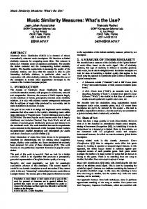
where we use ”W” to denote a break, or a time gap larger than a threshold T. In the work reported here we chose T to be 5 minutes. This indicates a break for commercials, news, traffic updates or another discontinuity in the EAS. From this we produce a graph by drawing an undirected arc between all adjacent objects; for example B is adjacent to A, G and D in the list. We denote the arc joining nodes X and Y by the unordered pair (X, Y ). Thus here, the arcs (B, G) and (B, D) would have weight one, while the arc (B, A) would have weight two. This is shown in Figure 1. This is repeated for all objects until we have represented all adjacencies by links on the graph. The graph we construct in Section 4 will have tens of thousands of nodes. A simple way to estimate similarities then flows
B F
1 G
2
1
1 A
1
E
S
1
2 K
1
1
D
1 J
Figure 1: Graph representing the labeled stream in (1). Songs represent nodes and adjacency increases the weight of the link between two nodes. from techniques to determine distances on graphs. The distance can be modeled as being inversely related to the weights on the graph. Thus A in Figure 1 will be closer to E than to other nodes on the graph. A very simple way to produce a playlist also follows. Start with a seed node, say, A. Choose the next objects from the set of objects that have arcs to A of weight at least one: SA = {B, E}. For example, a subsequent object may be chosen with likelihood proportional to the weight of the arc. Repeat this procedure on the newly chosen object. We will describe the actual algorithm used below. The contribution of this paper is to draw attention to a previously unexploited source of information: namely the order information in expertly authored streams. We show how this may be used to infer “likeness” between songs based on actual play patterns, rather than on any articulated rules or preferences or manually determined genre labelings. We show how to use this for an automatic playlist generation algorithm that scales to collections of millions of songs without difficulty. Compared to previous playlist generation methods our scheme has the advantage that it explicitly produces a measure of similarity between songs; it does not require access to a (human-generated) genre metadata database; the similarity measures improve automatically without human intervention as more data becomes available, and the scheme can handle very large collections easily.
2.
RELATED WORK
There has been significant recent growth in the research activity in the areas of multimedia content indexing and retrieval. We can give no more than a sampling of recent work in this area. Since our focus is primarily on song objects we will concentrate on recently reported work on playlist generation and music discovery.
2.1
Collaborative filtering
Collaborative filtering is often used to establish similarity and predict events when there is no natural idea of distance between objects. For example Amazon book recommendations compares users’ purchasing habits to recommend books to an individual based on purchases made by others with similar tastes. Generally this requires access to a large database of user data. Since for music this gives information at the album level rather than the track level it does not appear to have been applied successfully to playlist generation.
2.2
Audio content analysis
Several recently reported algorithms allow identification of music from a stream [6, 9]. These audio fingerprinting algorithms as they are known, enable identification of songs even after they have been compressed, companded or otherwise distorted over noisy channels. While they measure “similarity” in one sense they are not useful in determining that one song is “like” another. For example there is no expectation that the fingerprint of a particular song will be any closer to fingerprints of songs by the same artist, by similar artists, or of songs from the same genre than to a randomly selected song [6]. The question of genre detection from the audio content is expressly addressed by Tzanetakis and Perry in [15]. Using a combination of spectral and audio features the authors classify a collection into ten different genres. While the approach appears very promising for classification, a far finer selection of genres is necessary to make useful playlists or give a reliable measure of similarity. It is unclear whether audio genre classification techniques would be able to accurately classify hundreds of different sub-genres over a collection of tens of thousands of songs. A hierarchical approach for analysis and retrieval is presented by Zhang and Kuo [16]. Music is classified using such features as timbre and rhythm, and non-music sounds are classified at a higher stage. An excellent review of content-based genre classification algorithms is given by Li et al. [10].
2.3
Automatic Playlist Generators
There have been a number of recently reported approaches to the automatic playlist generation problem. Alghoniemy and Tewfik [4] describe a playlist generation system by posing it as a linear programming constraint satisfaction problem. Their system requires metadata on each of the songs in the collection indicating membership of various constraint sets. Pauws and Eggen [12] describe a system that employs dynamic clustering to group songs by metadata attribute similarity. Different weights for the various attributes are used to carefully balance the relative importance of various pieces of metadata. Platt et al. [14] employ a Gaussian
Process kernel to predict likely user playlists. This kernel is learned from a large set of album contents, which are used as sample playlists. Logan by contrast [11] generates playlists based on audio similarity measures. Audio information alone was reported to perform well on a database of size 8000 songs. One of Logan’s findings was that adding some metadata, such as genre information, considerably improved the performance of the system. The issue of scalability is directly addressed by Aucouturier and Pachet [5]. The authors point out that many playlist generation methods that work well for collections of a few hundred songs cannot be used as the collections grow to tens of thousands and beyond. By assigning various costs to the desired constraints they demonstrate generating playlists from a collection of 200000 songs. One of the significant advantages of our method is its scalability (see Section 4, also [13]). The approaches of [4, 12, 14] use meta-data such as is available in the All Music Guide database; that of [11] uses a combination of audio data and metadata. A completely different source of data is explored by Hauver and French in [8]. They use the history of requests being made to various internet radio stations. This request history is used to infer both artist popularity and pairwise similarities between artists. The next chosen song in a playlist is that by an artist that is both popular among the requesting audience, and similar to the artist of the last played song. Our approach is close in spirit to [8]; while we use an entirely different source of information our scheme also seeks to infer similarity from actual observed behavior on real streams rather than from genre information. Several of the playlists generation techniques [14, 11, 5, 4, 12] depend on a manually labeled database. While co-membership of such categories can be extremely useful, several of the classifications can be somewhat arbitrary, and the quantization into categories can be coarse and error-prone. By contrast our method depends only on what is actually played on real stations. It requires no manual labeling, and the estimates of “likeness” constantly improve as more data arrives. Thus any noise caused by capricious decisions by a DJ on a particular station quickly become averaged out in the stream of data.
3.
METHOD
We now describe our method for exploiting the similarity information that is implicit in an EAS. First, of course, we assume availability of a labeled summary of an EAS. We will discuss various sources in Section 3.1. The key assumption of our scheme is that songs that have appeared in close proximity in an EAS are more likely to be similar than those that have not. To take a concrete example, songs that appear on a Top 40 pop
radio station will appear somewhat alike: within this set those that have appeared adjacent will be judged closer together than those that have not. Most of the songs from the Top 40 pop station will be judged very unlike songs from a Jazz station, since most of them have never appeared in any proximity to the songs that play there. Songs that play on both the Top 40 pop and the Jazz station (such as some songs by “crossover” artists such as Sade, or Norah Jones) may appear close to several categories.
3.1
Sources of data
The heart of our method requires a summary of the EAS in labeled form. Having the song title and artist name is the simplest example, but all that matters is that we have an identifier that is unique to each song, the actual play order, and a method to identify gaps in the playlist (such as those generated, for example, by advertisements). For our experiments we used the Nielsen Broadcast Data Service (BDS) data; we briefly review other possible sources for those who might wish to replicate our approach and do not have access to that dataset.
3.1.1
Labeling provided from RDS
The Radio Data System is a protocol to provide metadata on the station and content over the FM broadcast channel. It is not universally used (e.g. it is not widely available in North America). Where it is available, a special decoder is needed to access the data.
3.1.2
Labeling obtained from station web-sites
The majority of terrestrial broadcast radio stations do not provide an accurate labeled list of the songs that they play. Most internet radio stations do, however. See for example the playlist tab on KEXP’s web-site [1], where they give access to all songs played in an archive that contains five years’ worth of music. Other stations such as RadioParadise [2] make available metadata lists for the last several hours of music. Thus, in principle, meta-data lists are available for several internet radio stations. In practice however screen scraping may violate the Terms of Use of a web-site, rendering the data unavailable for this purpose1 .
Artist Patsy Cline Sade ABBA The Beatles Shania Twain
Num. stations 120 238 220 326 403
Table 1: Sample artists and the number of stations on which they were played at least once. databases of millions of objects and still run in realtime on a desktop PC. A commercial service that identifies songs is available [3]. Training these schemes requires a labeled database.
3.1.4
Nielson Broadcasting Data
The BDS data monitors more than 1300 radio stations in the US and logs their entire playlists. For our experiments we used 36 days worth of the play order data from the BDS database. This consists of 1360 individual feeds, each of which contains the play order data from an individual broadcast radio station. Most of these are music stations that play predominantly pop music. Many of the stations play specialized mixes such as Top 40, Classic Rock, Oldies etc. while others play a mix. The feeds are a reasonably representative sampling of the radio stations broadcasting in North America. Some stations play as many as 2500 distinct songs, some play as few as 200. A total of 469,797 songs were played on all of the stations, of which 60,499 were distinct. Combining all of the EAS we thus get a graph that contains 60,499 nodes. Of these 33,251 appeared more than once. Table 1 gives a glimpse of the station coverage, listing several well-known artists and the number of stations (of the 1360 examined) that each of them appeared on at least once. Observe that cross-over artists appear on more stations than those confined to a single genre, even though this is not necessarily reflective of the amount of airtime they receive.
3.2
Building a Graph from an Ordered List
A very powerful set of audio finger printing algorithms allow identification of audio (or video) clips [6, 9]. These algorithms allow identification of a clip from a stream with audio objects in a labeled database. Thus, for example, they can listen to an FM over-the-air radio broadcast and output a list of the songs played together with timestamps. The successful algorithms can scale to
We now address the question of building a graph from an EAS. The labeled stream will be an ordered list of indices (cf. Figure (1)). We use this list to construct an undirected graph as follows: each object is a node in our graph. All weights are initialized to zero. When, for example, song B follows song A in the sequence, we increment the weight of the arc between them: WAB ← WAB + 12 . Thus for the simple example sequence in (1) we would get the graph shown in Figure 1. Call SA the set of all songs that have been adjacent to A at least
1 Readers are cautioned to always respect an internet radio station’s Terms of Use.
2 Note
3.1.3
Labeling the EAS using audio fingerprinting
that since the graph is undirected, WAB ≡ WBA .
once: SA = {X|WXA > 0}. Observe that the graph need not be fully connected. This is so since a time gap of greater than T (= 5 minutes, for example) between two objects does not count as adjacency. Thus a sequence of songs bracketed by such gaps might form a sub-graph disconnected from the rest if none of the songs appeared again. In general, however, the graph gets denser and more richly connected as time goes by, and more and more elements appear in the sequence. For the sequence generated from a single EAS we observe that the graph is almost always fully connected. It is often the case, however, that some objects occur infrequently in a certain stream and thus they are only weakly connected to the rest of the graph. We will give example statistics in Section 4.
3.2.1
Merging graphs from various different streams
For each of the EAS we form an undirected graph using the approach above. Since these streams tend to be specialized we must in general expect that no labeled stream covers more than a narrow subset of objects. For example a Pop 80’s station won’t include Country and Western. However as we include data from more EAS’s, the graphs will become more connected. We treat all EAS’s equally and every adjacency event in any of the labeled streams increases the weight by one. (There might be reasons why we would want to weight the contributions from different EAS differently; for example, the adjacency information from a less influential or popular station might be weighted lower than that of a very popular station.) Thus in our simplest model the overall graph formed using many labeled EAS’s would be the same as the one generated by concatenating them separated by time gaps greater than T.
3.3
Distances on graphs
The number of nodes in the graph is the number of unique objects that have occurred over the union of our labeled EASs. Some objects occur very often and some only once. Since our key assumption is that objects that occur in proximity to each other are more likely to be similar than those that do not, we desire a measure of “likeness” that decreases as the number of adjacency events between two objects increases. This is accomplished by mapping our undirected graph to a (directed) Markov random field, as follows. Consider some node A. Take all arcs terminating on A, sum their weights, and construct new directed arcs, all leaving A, with attached probabilities, which are just the original weights of the corresponding undirected arcs, divided by the sum of weights. Those probabilities are now transition probabilities, and the net probability of leaving node A is one. Do this for each node. Finally discard the
undirected arcs. Notice that this procedure results in each undirected arc (A, B) generating two corresponding directed arcs, one from A to B and one from B to A, and that due to the normalization procedure, the pair of arcs between a given pair of nodes may have different associated transition probabilities. The resulting graph is a Markov random field. In order to generate playlists, we simply perform a random walk, starting at the start node (song), and using the Markov transition probabilities. Now, we can map the probabilities to distances by replacing them by their negative logs. Thus, adding the distances of the arcs along a path amounts to computing a negative log likelihood for that path. To compute similarity between two songs, we then use the Dijksta algorithm [7] to compute the shortest path between those two songs. The similarity measure itself could then be, for example, the negative of the shortest distance (i.e. the log likelihood). If there is no path between a given pair of nodes (in the case of a nonconnected graph) we can define the distance to be some maximum value, larger than the diameter of the graph. The astute reader may at this point be asking, why not start with a directed graph? After all, the sequence of the songs as they are played defines a directional ordering; each transition from song A to song B would increment the weight of a directed arc from A to B. The problem is that such a scheme is more sensitive to asymmetry in playlists, which with limited data will occur by chance. For example, a given song B may directly follow another given song A several times, whereas A never follows B directly. In this case, using a directed graph computed directly from the original sequence will give a non zero probability of B following A, but a zero probability of A following B. In contrast, using our scheme described above, which constructs an intermediate undirected graph, encapsulates our belief that a sequence of two songs (A, B) in a playlist is more informative about the (symmetric) similarity of songs A and B than it is a statement that song B should always follow song A in any playlist.
3.4
Playlist Drift
Depending on the data set used to generate the graph, “drift” can be a problem for generated playlists. This occurs when successive steps in a walk of the song transitions result in an overall transition between two very unrelated areas. This is particularly prevelant at any steps that center on a song that crosses genres or audiences. Without additional information, that song cannot represent the aspect of the music that led to it. There are several ways to mitigate this. If the current state is extended to include the previous song, the degreee of drift introduced by a highly-connected song can be reduced. The distribution of songs contained in sequential playlist triplets that also contain the current
song and the previous song is much tighter in style. This can be extended indefinitely, of course, but it eventually degrades to matching only a particular radio station, approximately. The distribution of songs following the songs can also be a mix of that following the current song and that following the previous song, with some discount factor on the previous song. This simpler approach still mitigates the effects of choosing unlikely steps, and can also be extended as far as desired. A penalty function can directly bias a generated playlist towards the original seed or given list (such as a particular radio station). This minimizes overall drift. Local low-probability choices for individual songs can be eliminated by a cutoff on the number of times an arc must be observed in the source data in order to be present in the graph (although that will bias heavily towards songs that are frequently played).
4.
EXPERIMENTS
4.1
Examples Playlists
We now present a few sample playlists to illustrate the scheme. Each playlist is seeded by a single song, which is the starting point. The accompanying numbers represent the distance from the seed. Our first example starts with “Paperback Writer” by the Beatles: Paperback Writer [Beatles] Breakfast In America [Supertramp] We’re An American Band [Grand Funk Rrd] In The Dark [Billy Squier] I Shot The Sheriff [Eric Clapton] Fat Bottomed Girls [Queen] Jumpin’ Jack Flash [Rolling Stones] Working For The Weekend [Loverboy] Dream Weaver [Gary Wright] Smells Like Teen Spirit! [Nirvana] Can’t Stop [Red Hot Chili Peppers] Still Waiting [Sum 41] Grave Digger [Dave Matthews]
0.0 8.607 8.607 17.244 12 .192 16.335 13.723 15.251 15.520 15.735 16.732 19.256 20. 665
Note that the list stays within the broad category of music that could be considered close: for example it never strays into Jazz, Country, Hip Hop or Punk. Our next example is a Country song “Stand by Your Man” by Tammy Wynette: Stand By Your Man [Tammy Wynette] Chrome [Trace Adkins] Stay With Me (Brass Bed) [Josh Gracin] Whiskey Girl [Toby Keith] Class Reunion [Lonestar] My Sister [Reba McEntire] Could Have Fooled Me [Adam Gregory]
0.0 8.607 8.607 14.162 13.965 12.650 12.777
Nothin’ To Lose [Josh Gracin] Who’s Your Daddy [Toby Keith] Want Fries With That [Tim McGraw] Hell Yeah [Montgomery Gentry] Awful, Beautiful Life [Darryl Worley] Let Them Be Little [Billy Dean]
8.607 13.695 8.607 14.214 12.607 13.777
Again observe that the list stays entirely within the genre of Country music. Finally, starting with a Nirvana song: Lithium [Nirvana] : 0.0 Fall To Pieces [Velvet Revolver] 7.668 Tonight, Tonight [Smashing Pumpkins] 12.712 Slow Hands [Interpol] 12.712 Renegades Of Funk [Rage Against...] 10.127 Before I Forget [Slipknot] 7.355 The Kids Aren’t Alright [Offspring] 11.712 All These Things That I’ve Done [Killers] 9.542 Weapon [Matthew Good] 18.914 Kryptonite [3 Doors Down] 11.127 Home [Three Days Grace] 8.712 Whatever [Godsmack] 10.127 Colors [Crossfade] 7.097
4.2
Music Similarities
Our random walk playlist generation induces a desirable variety and unpredictability. However to evaluate our similarity measure, we also list the shortest path songs for a number of different seed songs. Note that the resulting playlists adhere much more closely to the seed song than the random walk playlists given above: Hey Jude [Beatles] Lady Madonna [Beatles] Lucy In The Sky With Diamonds [Beatles] Peace Of Mind [Boston] (Just Like) Starting Over [John Lennon] Saturday In The Park [Chicago] Shine It All Around [Robert Plant] Holiday [Green Day] Rock And Roll Heaven [Righteous Brothers] Highway To Hell [AC/DC] Best Of You [Foo Fighters] Remedy [Seether] Right Here [Staind] Holiday [Green Day] Be Yourself [Audioslave] The Hand That Feeds [Nine Inch Nail s] B.Y.O.B. [System Of A Down] Happy? [Mudvayne] Shine It All Around [Robert Plant]
0.000 7.515 7.515 7.737 7.737 8.000 8.000 8.000 8.000
0.000 6.252 6.362 6.362 6.362 6.5 58 6.584 6.754 6.847 6.982
Stand By Your Man [Tammy Wynette] You’ll Be There [George Strait]
0.000 5.800
Stand By Your Man (Wynette) Achy Breaky Heart (Cyrus) Hey Jude (Beatles) Paperback Writer (Beatles) Highway To Hell (AC/DC) Lithium (Nirvana) I Wanna Be Sedated (Ramones) Intergalactic (Beastie Boys) Just A Lil Bit (50 Cent) Straight Outta Compton (NWA)
Stand By Your Man
Achy Breaky Heart
Hey Jude
Paperback Writer
Highway To Hell
0
14.737
18.917
18.515
14.012
0
17.696
20.631
20.136
18.515
Lithium
I Wanna Be Sedated
Intergalactic
Just A Lil Bit
Straight Outta Compton
17.509
19.316
21.214
23.681
18.145
29.095
19.896
16.893
17.656
18.741
20.843
13.686
23.808
0
10.322
15.552
15.492
17.077
17.98
14.845
27.263
20.621
8.607
0
14.982
15.955
15.982
17.136
14.452
24.962
21.241
21.349
17.569
18.714
0
9.532
12.339
12.339
13.207
27.312
23.421
22.485
17.882
20.06
9.905
0
10.712
11.127
12.815
26.317
23.985
22.236
18.133
18.753
11.378
9.378
0
9.793
13.468
21.51
26.055
23.942
18.64
19.51
10.982
9.397
9.397
0
12.522
23.698
26.441
22.707
21.426
22.748
17.771
17.007
18.994
18.444
0
15.319
27.216
22.654
23.669
23.082
21.7
20.332
16.86
19.444
5.143
0
Table 2: Similarities between sampled songs from the dataset. Highwayman [Highwaymen] Making Memories Of Us [Keith Urban] Play Something Country [Brooks and Dunn] If I Said [Bellamy Brothers] Alcohol [Brad Paisley]
5.800 6.022 6.022 6.022 6.022
will also weigh heavily towards popular artists. If this is not the desired behavior, the weight contributions can be normalized by dividing by the number of total ocurrences of the adjacent song. This produces lists of similar artists such as: Tammy Wynette Don Williams Prairie Oyster Gatlin Brothers
Table 2 shows the similarity distances that our graph produces for a sampling of different songs chosen from across the spectrum of genres. Observe that songs by the same artist are much closer together than either are to those from other genres. Also note that the similarity matrix is not symmetric, since the graph is directed (see Section 3.3).
4.3
50 Cent Eminem Jay-Z 2Pac Ludacris
Artist Similarities
The generality of this graph-based method allows for other connections to be draw between the entities. An interesting application is determining similar artists. This can be performed by simply considering artists to be similar when their songs are frequently played next to each other. The song graph is transformed into one where there are edges between artists, annotated with weights of the number of times the artists at the endpoints have and instance of a song from each occuring adjacently. This can then be used as before to generate transition probabilities and distances between artists. In practice, it is useful when computing the artist edges to ignore songs that only occurred once (or very few times), since they will add noise. This procedure
0.00 2.00 4.34 4.36
0.00 6.03 6.25 6.73 6.93
The similarity distances for the artists of the songs used as examples earlier are shown in Table 3. Note that artists of similar genres and styles are closer together.
5.
CONCLUSION
We have proposed a scheme to infer similarities between songs, and to generate playlists automatically. Like other methods, our process relies on the availability of human-generated metadata. However, while gathering such data is normally an expensive proposition, the data we use is already readily available, for a very large number of songs, in the form of radio station playlists. Fur-
Tammy Wynette Billy Ray Cyrus Beatles AC/DC Nirvana Ramones Beastie Boys 50 Cent NWA
Tammy Wynette
Billy Ray Cyrus
Beatles
AC/DC
Nirvana
Ramones
Beastie Boys
50 Cent
NWA
0.00
14.56
13.55
18.00
17.99
16.62
17.78
23.33
26.59
11.77 14.94 17.98 18.31 15.61
0.00 19.37 18.36 21.39 19.13
13.13 0.00 6.74 11.60 10.50
19.33 8.87 0.00 6.61 9.42
20.49 14.67 7.75 0.00 7.63
19.94 11.75 12.53 9.09 0.00
22.32 15.75 10.49 7.83 7.16
21.38 18.82 16.06 16.44 17.35
25.46 19.52 16.56 13.70 16.95
18.72 19.16 21.34
21.50 21.98 24.72
12.28 14.29 16.05
9.33 15.71 16.27
7.77 16.23 11.42
10.72 17.72 17.64
0.00 13.27 12.95
10.19 0.00 10.80
9.79 9.22 0.00
Table 3: Similarities between sampled artists from the dataset. thermore, explicitly authored metadata for songs can be very noisy (for example, opinions can differ widely as to which sub-sub-genre a given song should belong). Playlists, on the other hand, are carefully designed by experts with a strong economic incentive to retain listeners. We have demonstrated that such data can easily be used to form a Markov random field. This can then be used to generate new playlists, by executing a random walk from the seed song. A corresponding graph where probabilities have been mapped to negative log likelihoods can be used to compute the similarity of any pair of songs, by computing the shortest distance between their corresponding nodes. Such paths can also be used to generate playlists with given start and end songs, which gives the user control over how the playlists changes over time (for example, from upbeat, fast music to slow music). Our proposed scheme is very general. It can be used to generate playlists in the style of a given radio station, by constructing a graph from only that station’s playlists. It can also be used for a music recommendation system by constructing the graph from all available data and using the songs/artists in a given user’s library as starting nodes. The method proposed is very fast. Updating the system as new data becomes available amounts to simply adjusting counts on the arcs. Human intervention is required only in the original construction of the radio station playlists, so the system can improve automatically over time (in both coverage, and in the estimates of similarities) as more playlist data becomes available. Playlist data can either be obtained directly from the content providers or by using automated monitoring systems, such as audio fingerprinting systems. Similar schemes could be used for other media which occurs in authored streams, such as music videos.
6.
[1] [2] [3] [4] [5] [6] [7] [8]
[9] [10] [11] [12]
[13] [14]
[15] [16]
REFERENCES
http://www.kexp.org. http://www.radioparadise.com. http://www.shazam.com. M. Alghoniemy and A. H. Tewfik. A network flow model for playlist generation. Proc. ICME, 2001. J. J. Aucouturier and F. Pachet. Scaling up playlist generation systems. Proc. ICME, 2002. C. J. C. Burges, J. C. Platt and S. Jana. Distortion descriminant analysis for audio fingerprinting. IEEE Trans. on SAP, 11, 2003. T. H. Cormen, C. E. Leiserson, and R. L. Rivest. Introduction to Algorithms. McGraw Hill, 1990. D. B. Hauver and J. C. French. Flycasting: using collaborative filtering to generate a playlist for online radio. Proc. Int. Conf. Web Delivering of Music, 2001. J. Haitsma and T. Kalker. A highly robust audio fingerprinting system. Proc. Intl Conf on Music Information Retrieval, 2002. T. Li, M. Ogihara, and Q. Li. A comparative study on content-based music genre classification. SIGIR, 2003. B. Logan. Content-based playlist generation: Exploratory experiments. Proc. Third Intl. Conf. on Music Information Retrieval, 2002. S. Pauws and B. Eggen. PATS: Realization and Evaluation of an Automatic Playlist Generator. Proc. 3rd International Simposium on Music Information Retrieval, 2002. J. Platt. Fast embedding of sparse music similarity graphs. NIPS, 16, 2004. J. C. Platt, C. J. C. Burges, S. Swenson, C. Weare, and A. Zheng. Learning a gaussian process prior for automatically generating music playlists. NIPS, 2001. G. Tzanetakis and P. Cook. Musical genre classification of audio signals. IEEE Trans. on SAP, 10(5), 2002. T. Zhang and C.-C. Jay Kuo. Hierarchical classification of audio data for archiving and retrieving. Proc. IEEE ICASSP, 1999.