A Simple and Efficient Optimization Routine for Design of ... - CiteSeerX
Recommend Documents
Key words: Semidefinite Programming, large sparse problems, inexact Gauss-Newton ...... tolerance 1.0e-01; optimal values of order 150; SUN computer.
dollars) and several hours of processing time, and results in highly variable recoveries .... including three 50 l samples and one 100 l sample by TFF and four 20l ...
T. Blumensath and M. E. Davies. IDCOM & Joint ... Iterative Hard Thresholding, has near optimal performance guaran- ... tish Funding Council and their support of the Joint Research Institute with ... able in our technical report on arXiv [5]. 2.
T. Blumensath and M. E. Davies. IDCOM & Joint Research ... Iterative Hard Thresholding, has near optimal performance guaran- tees rivalling those ... tish Funding Council and their support of the Joint Research Institute with the Heriot-Watt ...
Feb 9, 2005 - Development and application of a simple routine method for the determination of selenium in serum by octopole reaction system ICPMS.
Morrison, J. L., 1980, Computer technology and cartographic change. In Taylor, D., editor, The. Computer in Contemporary Cartography. J. Hopkins Univ. Press ...
for dealing with several well-known problems with elementary constraints such as SAT, frequency assignment ..... ËAbo Akademi University. ⢠Department of Computer ... Turku School of Economics and Business Administration. ⢠Institute of ...
each polyline, and use them as input to general map-labeling algorithms as ... on the number of points of the polyline, and not on other parameters such as the ... A special case arises if ti lies in the interior of the ε-buffer. ... point or edge t
detection together with raising fourth power of the signal to cancel QPSK modulation format is applied. However, initial timing offset is required to be within.
IEEE 802.11 wireless LAN (WLAN) [1] has gained a great success for data applications in hotspots, en- ... Recent performance evaluations of 802.11e HCF [4].
formation of diazonium salt was confirmed by a test with β-naphthol. When the diazotization was complete, potassium iodide (5 mmol) was added to the paste- ...
Mar 26, 2014 - To optimize the γ-ray beam quality, an optical system preserving ..... top view of Fig. .... recirculator with the CODE V software [37] (128 reflective.
of a building's facade when several parameters are allowed to change ... maintaining good daylight penetration. The results ... effectively for facade design optimization considering ..... workshop4/cd/website/PDF/ Ward_rtcontrib.pdf. Wienold J.
Mar 12, 2016 - 180 kg payload. 75 kg vertical stab. 6 kg horizontal stab 1 and 2. 12 kg. 57. ê±´êµëíêµ | IP: 203.252.161.96 | Accessed 2016/03/12 01:01(KST) ...
Aug 12, 2010 - Structure of 6,6'-dibromoindigo (1, Tyrian purple). 1. N. N. O. O. Br. Br. H ... The traditional syntheses of 6 involve the use of p-toluidine [5], o-nitrotoluene [6], .... Since it turned out that 4-bromo-2-chlorobenzoic acid (18) did
During last decades sport activities for disabled people are practiced by many and many athletes, both amateurs and professionals. In order to give the ...
Summary: The molecular weight analysis of urinary proteins can provide useful diagnostic .... The main part of the gel production device was the gel casting.
ETH Zurich, Switzerland [email protected]. Vijay Menon. Google. Seattle, WA ... leveraging existing dynamic optimization infrastructure in a Java ...
1620s. 5582s. 16.16.16. 84736. 326400. 6363s. 11000s. 16.32.4. 71424. 193280 ...... In Proceedings of SIGCOMM 94, London, England, 1994. 73] S. Sibal and ...
tween a given input order and the required order a given al- ... They introduced cost-based query optimization. Based on some cost model ... derings, consider a tuple stream that is sorted on some at- ... the attribute sequence (a, b) and (b, a) or e
Page 1. Adapting Query Optimization Techniques for Efficient ..... adapting database query optimization techniques, including various main memory index ...
parameters in the protocol software implementation, we can shape the activity ... For example, the wake-up time of a Cisco Aironet wireless LAN card is almost twice the .... By monitoring the TCP receive buffer occupancy or utilization, we want ...
from the DEFCON 8 CTF dataset, it took the DBMS-based alert correlator around ... of experiments to evaluate these techniques with the DEF CON 8 CTF data.
A Simple and Efficient Optimization Routine for Design of ... - CiteSeerX
transformers. Minimizing the product of power loss, core cross section and winding area is chosen as the optimization goal. This object function leads to a closed ...
A Simple and Efficient Optimization Routine for Design of High Frequency Power Transformers
Shahrokh Farhangi
A Simple and Efficient Optimization Routine for Design of High Frequency Power Transformers Shahrokh Farhangi Amir-Abbas Shayegan Akmal DEPT. of ELECT. and COMPUTER ENG. UNIVERSITY of TEHRAN North Kargar Ave. Tehran-Iran [email protected]
Keywords Magnetic Devices, Passive components, Modelling,
Abstract An efficient, meanwhile simple optimization routine is presented for design of high frequency power transformers. Minimizing the product of power loss, core cross section and winding area is chosen as the optimization goal. This object function leads to a closed form solution, which reduces the computation time and the number of iterations. A CAD tool has been developed according to this method, which is addressed in this paper. By this tool the optimized core which fulfills the temperature rise constraint is determined. If the area product of the selected core is bigger than the optimum area product, the user can modify his design further by minimizing the power loss. The validation of the method is verified by a sample design example.
1. Introduction The main objectives in optimization of high frequency power transformers are minimizing volume, weight, power loss and cost. Availability of various types and sizes of cores, complexity of power loss models, vast and various range of design requirements, make optimum manual design difficult and time consuming. Therefore, several researchers have paid attention to develop computerized optimization routines for design of magnetic components in recent years [1], [2], [3]. In [3] the transformer power loss has been used as an object function, and a detailed thermal model, based on one dimensional steady-state heat transfer, has been used to derive the core and winding temperature rises. In this paper the product of power loss, core effective area and winding area is used as the optimization index. Instead of a detailed thermal model, Williams' model [4], which relates the power loss of the component to its average surface temperature, is used. The optimization procedure has two stages. At first stage the optimum core size is determined. At the second, the windings are modified, in order to minimize the power loss. At both stages, the optimum flux and current densities are derived in closed form. It is shown, that accuracy of the proposed routine is good enough. The core loss, winding loss and thermal models are described at Section 2. The mathematical basis of the routine is discussed in Section 3. The structure of the optimization process is presented in Section 4. To check the validity of the models, and the accuracy of the CAD tool, sample designs are presented in Section 5, and the results are discussed. Section 6 concludes the paper.
2. Power Losses and Thermal Models 2.1 Core Loss The core loss for ferrite cores is expressed as:
EPE '99 - Lausanne
P. 1
A Simple and Efficient Optimization Routine for Design of High Frequency Power Transformers
Pcore = c mVcore f m Bmn
Shahrokh Farhangi
(1)
Where Pcore is the core loss in watt, Vcore is the core volume in m3, f is the working frequency in Hz, Bm is the amplitude of flux density in Tesla and cm is a constant. cm, m and n can be found from the core data sheets [5].
2.2 Copper Loss The copper loss is the sum of ohmic losses of all windings. For a transformer with two windings, it is calculated as follows: 2
2 PCu = ∑ FR ( xi ) Rdc (i ) I rms (i )
(2)
i =1
Where Rdc = ρ lmean /ACu, and FR(x) = Rac / Rdc is the ratio of ac to dc resistance. The Dowell model [6] is used in this paper for interpretation of ac resistances. Because it is in closed form and well accepted among researchers [2], [3], [7]. For a winding made of copper foil it is written as:
2( M 2 − 1) FR ( x) = x G ( x) + H ( x) 3
(3)
Where:
G ( x) =
sinh 2 x + sin 2 x cosh 2 x − cos 2 x
(4)
H ( x) =
sinh x − sin x cosh x + cos x
(5)
In (3) x =
K layer , M is the number of layers from zero to maximum amper-turns, δ = 2 ωσµ ,
h δ
is the skin depth, h is the foil thickness. Klayer = NL b / bw is the layer utilization factor. Where NL and b are the number of turns and width of a filled layer, respectively, and bw is the width of the core window.
For a winding made of Litz wire, the equation (3) should be modified as follows [7]:
2( M 2 N s − 1) FR ( x) = x G ( x) + H ( x) 3 Where x =
ds 2δ
(6)
πK layer , K layer = πN s d s d L . Ns, ds and dL are the number of strands, strand
diameter and overall diameter of Litz wire, respectively. For a winding which has M complete layers, and the M+1 layer is partially filled, with Np number of turns, (6) is modified as follows [8]:
[(
)
2 FR ( x) = x G ( x) + M 2 N s − 1 + 3
EPE '99 - Lausanne
N p Ns NL
(2M + 1)] H ( x)
(7)
P. 2
A Simple and Efficient Optimization Routine for Design of High Frequency Power Transformers
Shahrokh Farhangi
The copper loss for a non-sinusoidal waveform can be derived from (2) to (7) by expanding the current waveform into Fourier series: 2
PCu =∑ i =1
K
∑R k =1
2 ac ( ik ) rms ( ik )
I
(8)
Where K=50 is used in this paper.
2.3 Thermal Model Williams' thermal model is used for determining the temperature rise of magnetic components [5]:
1000 δθ = 59 θa
1.69
Ploss A surface
0.82
(9)
In this equation δθ is the average surface temperature rise of the magnetic component (in oC), θa is the ambient temperature (in oC), Ploss is the total power loss (in W), and Asurface is the external surface area of the core and winding (in cm2). This equation is based on experimental results. It does not specify the hottest point of the device. Usually, the temperature difference between the hottest point and the surface of the magnetic component does not exceed a few degree centigrade (except at very large devices). Therefore, it can be used with enough accuracy, which is needed during design stage of these components.
3 Optimization Routine 3.1 Core Optimization The product of core cross section, winding area and power loss is used as the object function. For a transformer with two windings the product of core cross section and winding area, which is known as area product, is expressed as follows:
Acore Awinding =
V1 I 1 + V2 I 2 K v K u Bm J w f
(10)
The power loss of the transformer is written as:
Ploss = FR ( x1 ) Rdc1 I 12 + FR ( x 2 ) Rdc 2 I 22 + c mVcore f m Bmn
(11)
Using (10) and (11) the object function can be expressed as:
F ( Bm , J w ) =
[
V1 I 1 + V2 I 2 FR ( x1) ρ1l mean1 Kv Ku f + c mVcore f m Bmn −1 J w−1
N1 I 1 Bm
+ FR ( x 2 ) ρ 2 l mean 2
N2I 2 Bm
(12)
]
In this equation Vi and Ii are the primary and secondary voltages and currents, Kv is a constant related to voltage wave-shape (4.44 for sinusoidal and 4/D for quasi-square wave-shape), Ku is the window utilization factor, and Jw is the common current density of the primary and secondary windings. Considering N1 I1 = N2 I2 and N1 = V1 / (Kv f Bm Acore), the equation (12) is simplified further as:
EPE '99 - Lausanne
P. 3
A Simple and Efficient Optimization Routine for Design of High Frequency Power Transformers
F ( Bm , J w ) =
V1 I 1 + V2 I 2 {[FR ( x1) ρ1l mean1V1 I 1 + FR ( x2 ) ρ 2 l mean 2V2 I 2 ] K v fA1core Bm2 Kv Ku f + c mVcore f B m
n −1 m
J
−1 w
}
Shahrokh Farhangi
(13)
In (13), after selecting the core, all variables are almost fixed, except Jw and Bm. This equation shows that by increasing Jw, the object function decreases. Therefore, Jw should be determined from another constraint, which is the required temperature rise. But (13) in relation with Bm has a minimum. The optimized value of flux density, which leads to this minimum, is derived as follows: 1
Bm ( opt )
2K1 n +1 Jw = (n − 1) K 2
(14)
Where K1 and K2 are defined as:
K1
∑ =
2 i =1
FR ( xi ) ρ i l mean (i )Vi I i
(15)
K v fAcore
K 2 = c mVcore f
(16)
m
Inserting Bm(opt) from (15) into the expression of the total power loss, the total loss is written as: (17)
n
1
Ploss = K 3 K 2n +1 ( K 1 J w ) n +1 Where K3 is defined as: n
1
n − 1 n +1 2 n +1 K3 = + n −1 2
(18)
From (17) the value of Jw can be derived:
1 Ploss Jw = 1 K 1 K K n +1 3 2
n +1 n
(19)
If the core and temperature rise is known, the total power loss can be specified from (9), therefore Jw and Bm(opt) can be determined from (19) and (14). Using the relations derived in this sub-section, the optimum core can be selected through a computerized routine, which is described in the next section.
3.2 Power Loss Minimization The optimization process specifies a core size, which fulfills the temperature rise constraint, and minimizes the optimization index. Since the ferrite cores are produced in certain types and sizes, the computerized routine finds the smallest core, with the area product equal or bigger than the optimum value. When the area product of the selected core is equal to the optimum value, the optimization routine will terminates. But, if it is bigger than the optimum value, then the winding can be changed in order to minimize the power loss. In this stage the core is fixed, and the power loss should be minimized. The equation (11) can be written as follows:
EPE '99 - Lausanne
P. 4
A Simple and Efficient Optimization Routine for Design of High Frequency Power Transformers
Ploss = K 1
Jw + K 2 Bmn Bm
Shahrokh Farhangi
(20)
In equation (20), after specifying the core, K2 is fixed, and K1 is almost fixed. Differentiating (20) with respect to Bm, gives the optimum value of the flux density, which minimize the power loss: 1
K n +1 Bm = 1 J w nK 2
(21)
The lowest value of Jw is found by assuming that the window is full:
Awindow =
N1 I1 N I + 2 2 K u1 J w K u 2 J w
(22)
Where Ku1 and Ku2 are the window utilization factors for the primary and secondary windings (Since V they may be maid of different conductor types.). Using N i = K v fBmi Acore and (21) results:
1 Jw = K fA v p
2
Vi I i ∑ i =1 K ui
n +1 n+2
nK 2 K1
1
n+2
(23)
Where, Ap is the area product of the core. Inserting Jw from (23) into (21) gives the optimum value of the flux density according to the core and transformer parameters:
Bm ( opt )
K = 1 nK 2
1
1
n +1 1 K v fA p
2
Vi I i ∑ i =1 K ui
n2
(24)
In deriving (23) and (24), it was assumed that K1 is fixed. This is not exactly true. Actually, K1 increases by decreasing Jw. But, it is not too sensitive with respect to Jw, and can be assumed be constant.
4 CAD Tool Structure 4.1 Design Procedure A software has been written in Visual Basic 4.0, which designs and analyses high frequency power transformers. The data of ferrite cores and parameters of common magnetic materials are stored in core data libraries. The design stage begins with reading of transformer requirements. The flowchart of optimum core selection is shown in Fig. 1-a. The type of the core and the grade of the magnetic material should be specified by the user. The program finds an initial core size, using the default values for Bm and Jw. The power loss is calculated for this core with the given temperature rise constraint. Then Jw and Bm(opt) is derived using (19) and (14), and the optimum value of area product using (10). If the optimum area product is bigger than the area product of the selected core, then a bigger core will be chosen. If the optimum area product is less than the area product of the selected core, then a core with one size smaller will be checked. The process of optimization terminates, when the optimum area product is smaller than the area product of the selected core, and bigger than the area product of a core with one size smaller. After selection of the proper core, the user can modify his design by minimizing the power loss.
EPE '99 - Lausanne
P. 5
A Simple and Efficient Optimization Routine for Design of High Frequency Power Transformers
Shahrokh Farhangi
Start Design Requirements Core Type and Grade Temperature Rise Start
5. Conclusion A design procedure has been presented in this paper for optimization of ferrite high frequency power transformers. The product of power loss, core cross section and winding area has been chosen as the optimization index, along with average surface temperature rise as the constraint. A CAD tool has been introduced, based on this optimization goal, which selects the optimum core , and provides the transformer parameters. After selection of the core, the designer can modify his design further by power loss minimization. In this stage of design the windings completely fill the window, but higher efficiency is achieved. The performance of the transformer, at operating conditions other than nominal, can also be investigated by this tool. The accuracy of modelling and design routine has been verified by experiment.
References 1. J. Jongsma. High frequency ferrite power transformer and choke design, Philips Tech. Pub., No 267, Philips, 1986. 2. P. M. Gradzki, M. M. Jovanovic, F. C. Lee. Computer aided design for high frequency power transformers, .IEEE PESC'90, pp. 336-343, 1990. 3. R. Petkov. Optimum design of a high power, high frequency transformer, IEEE Trans. on Power Electron. pp. 33-42, 1996. 4. B. W. Williams, Power electronics: devices, drivers, applications and passive components, 1992. 5. S. A. Mulder, Loss formulas for power ferrites and their use in transformer design, Philips Components, 1994. 6. P. Dowell. Effect of eddy currents in transformer windings, IEE Proc., vol. 113, pp. 1387-1394, 1966. 7. W. J. Gu, R. Liu, A study of volume and weight vs frequency for high frequency transformers, in Proc. IEEE PESC, pp. 1123-1129, 1993. 8. A. Shayegan Akmal, Optimized design of high frequency power inductors and transformers, M.Sc. Thesis, University of Tehran, 1998. 9. S. Farhangi, A. Shayegan Akmal, Design and optimization of transformers with ferrite cores, in Proc. ICEE, vol. 5, pp. 7-12, 1998.