efficient continuous algorithms for combinatorial optimization - CiteSeerX

EFFICIENT CONTINUOUS ALGORITHMS FOR COMBINATORIAL OPTIMIZATION

a dissertation submitted to the department of computer science and the committee on graduate studies of stanford university in partial fulfillment of the requirements for the degree of doctor of philosophy

By Anil Kamath June 1995

c Copyright 1995 by Anil Kamath All Rights Reserved

ii

I certify that I have read this dissertation and that in my opinion it is fully adequate, in scope and quality, as a dissertation for the degree of Doctor of Philosophy. Serge A. Plotkin (Principal Advisor)

I certify that I have read this dissertation and that in my opinion it is fully adequate, in scope and quality, as a dissertation for the degree of Doctor of Philosophy. Rajeev Motwani

I certify that I have read this dissertation and that in my opinion it is fully adequate, in scope and quality, as a dissertation for the degree of Doctor of Philosophy. Andrew Goldberg

Approved for the University Committee on Graduate Studies:

iii

Abstract The thesis concentrates on design, analysis, and implementation of ecient algorithms for large scale optimization problems with special emphasis on problems related to network

ows and routing in high-speed networks. The main focus is on using continuous techniques for solving large combinatorial optimization problems in o-line and online settings. Some of the major areas of work include:

Developing and implementing new interior-point techniques for eciently solving large scale multi-commodity network ow problems. These algorithms are based on solving linear and quadratic programming formulations of the problem.

Designing fast algorithms based on continuous methods for approximate solution of

minimum cost multi-commodity ow problem. These techniques are geared towards distributed implementation.

Application of multi-commodity ow techniques for design and implementation of centralized and distributed algorithms for on-line routing of Virtual Circuits in ATM (Asynchronous Transfer Mode) networks.

Our approach is to design algorithms that have provably good worst or average case performance and demonstrate their eciency by implementing and evaluating them on real data.

iv

Acknowledgements First, I would like to thank my advisor Serge Plotkin. He made my stay in Stanford exciting and stimulating. He provided ideas, advice and support throughout my Ph.D. work and this thesis would not have been possible without his guidance. Next, I would like to thank Rajeev Motwani for teaching excellent courses during my stay at Stanford and also providing me the opportunity for doing some interesting work with him. I also owe thanks to Andrew Goldberg for teaching interesting classes. I am grateful to Omri Palmon for collaborating on many parts of this thesis. His con dence and insight helped me a lot in my work. I would also like to thank K.G. Ramakrishnan, Narendra Karmarkar and Rainer Gawlick who co-authored some of the results presented here. Ramakrishnan provided the practical and implementational framework for most of the work in this thesis. He provided us with information and data on many interesting real-world problems. And many thanks to Birdy for being always willing to listen and ask probing questions about my work and tell me about the exciting work in his eld. I was also fortunate to have many interesting and helpful friends in the Computer Science Department, like Luca, Henny, Sanjeev, Julien, Jerey to name a few. Finally, I thank my parents, Prabhakar and Poornima, and my sisters, Swati and Sharmila, for their love and support. This research was supported by NSF Grant CCR-9304971 and ARO Grant DAAH0495-1-0121.

v

Contents Abstract

iv

Acknowledgements

v

1 Introduction

1

2 A Linear Programming method for the Multi-commodity Problem

6

2.1 2.2 2.3 2.4 2.5 2.6 2.7

Introduction : : : : : : : : : : : : : : : : : : : : : : : : : : : : Linear Programming Formulation : : : : : : : : : : : : : : : : An Overview of the Approximate Dual Projective Algorithm Complexity of ADP Algorithm for MCNF : : : : : : : : : : : Ecient Implementation of ADP Algorithm for MCNF : : : Concurrent Flow Problem : : : : : : : : : : : : : : : : : : : : Computational Experience : : : : : : : : : : : : : : : : : : : :

: : : : : : :

: : : : : : :

: : : : : : :

3 A Quadratic Programming approach to Multi-Commodity Flow

: : : : : : :

: : : : : : :

: : : : : : :

: : : : : : :

: : : : : : :

Introduction : : : : : : : : : : : : : : : : : : : : : : : : : : : : : : : : : : : : Multi-commodity ow as QP : : : : : : : : : : : : : : : : : : : : : : : : : : The Algorithm : : : : : : : : : : : : : : : : : : : : : : : : : : : : : : : : : : Analysis of number of operations per iterations : : : : : : : : : : : : : : : : 3.4.1 Computing the Newton step using conjugate gradient. : : : : : : : 3.4.2 Computing the Newton step using matrix inversion and rank one updates. : : : : : : : : : : : : : : : : : : : : : : : : : : : : : : : : : 3.5 Starting Point For The Algorithm : : : : : : : : : : : : : : : : : : : : : : : 3.6 Stability : : : : : : : : : : : : : : : : : : : : : : : : : : : : : : : : : : : : : : 3.7 Finding an Exact Solution : : : : : : : : : : : : : : : : : : : : : : : : : : : : 3.1 3.2 3.3 3.4

vi

6 7 8 12 13 16 16

19

19 22 23 27 28

31 33 35 37

3.8 Extensions : : : : : : : : : : : : : : : : : : : : : 3.8.1 Minimum Cost Multi-commodity Flow. 3.8.2 The Concurrent Flow Problem. : : : : 3.8.3 The Generalized Flow Problem. : : : :

: : : :

: : : :

4 Distributed Algorithm for Multi-commodity Flow 4.1 4.2 4.3 4.4 4.5

Introduction : : : : : : : : : : : : : : Preliminaries and De nitions : : : : The Flow Without Costs : : : : : : : Flow With Costs : : : : : : : : : : : Implementation of a single iteration

: : : : :

: : : : :

: : : : :

: : : : :

: : : : :

: : : : :

: : : : :

: : : : :

: : : : : : : : :

: : : : : : : : :

: : : : : : : : :

: : : : : : : : :

: : : : : : : : :

: : : : : : : : :

: : : : : : : : :

: : : : : : : : :

5 Approximate Algorithm for Min-cost Multi-commodity Flow 5.1 Introduction : : : : : : : : : : : : : : : : : : : : 5.2 Continuous algorithm : : : : : : : : : : : : : : 5.2.1 The Algorithm : : : : : : : : : : : : : : 5.2.2 Bounding number of phases : : : : : : : 5.3 Improving The Running Time : : : : : : : : : : 5.4 Bounding the number of phases of Algorithm-2

: : : : : :

: : : : : :

: : : : : :

6 Routing and Admission Control of Virtual Circuits 6.1 Introduction : : : : : : : : : : : : : : : : : : : : : 6.1.1 Previous work : : : : : : : : : : : : : : : : 6.2 Centralized On-line Algorithm for SVC Routing : 6.2.1 Exponential-cost based routing : : : : : : 6.2.2 Adding probabilistic assumptions : : : : : 6.2.3 Simulation Results : : : : : : : : : : : : : 6.3 Distributed Algorithm : : : : : : : : : : : : : : : 6.3.1 Simulation Results : : : : : : : : : : : : : 6.4 Discussion : : : : : : : : : : : : : : : : : : : : : :

: : : : : : : : :

: : : : : : : : :

: : : : : :

: : : : : : : : :

: : : : : :

: : : : : : : : :

: : : : : :

: : : : : : : : :

: : : : : :

: : : : : : : : :

: : : : : :

: : : : : : : : :

: : : : : :

: : : : : : : : :

: : : : : :

: : : : : : : : :

7 Competitive routing under known Holding time Distributions

: : : : : : : : : : : : : : : : : : : : : : : :

: : : : : : : : : : : : : : : : : : : : : : : :

: : : : : : : : : : : : : : : : : : : : : : : :

: : : : : : : : : : : : : : : : : : : : : : : :

: : : : : : : : : : : : : : : : : : : : : : : :

: : : : : : : : : : : : : : : : : : : : : : : :

7.1 Introduction : : : : : : : : : : : : : : : : : : : : : : : : : : : : : : : : : : : : 7.2 Notation and De nitions : : : : : : : : : : : : : : : : : : : : : : : : : : : : : 7.3 Adaptive Adversary : : : : : : : : : : : : : : : : : : : : : : : : : : : : : : : vii

38 38 41 45

47

47 49 50 53 56

58

58 60 61 62 66 69

72

72 74 78 78 80 83 90 91 93

95

95 96 97

7.4 Admission Control and Routing Algorithm : : : : : : : : : : : : : : : : : : 98 7.5 Exponential Holding Time : : : : : : : : : : : : : : : : : : : : : : : : : : : : 101 7.6 Simulation Results : : : : : : : : : : : : : : : : : : : : : : : : : : : : : : : : 103

Bibliography

105

viii

List of Tables 2.1 Performance of ADP on rmfgen problems : : : : : : : : : : : : : : : : : : : 2.2 Performance of ADP on the concurrent ow problem : : : : : : : : : : : : : 2.3 Performance of ADP on mgrid problems : : : : : : : : : : : : : : : : : : : :

17 18 18

6.1 NSFNet Trac Pro le : : : : : : : : : : : : : : : : : : : : : : : : : : : : :

88

ix

List of Figures 2.1 Pictorial View of the Approximate Dual Projective(ADP) Algorithm : : : : 2.2 MCNF Matrix : : : : : : : : : : : : : : : : : : : : : : : : : : : : : : : : : : 2.3 Object Oriented Structure of the Software : : : : : : : : : : : : : : : : : : :

9 14 14

3.1 Comparison of Complexities. : : : : : : : : : : : : : : : : : : : : : : : : : :

20

6.1 6.2 6.3 6.4 6.5 6.6 6.7 6.8

The original AAP routing algorithm : : : : : : : : Topology for an existing commercial network. : : : Simulation results for the centralized algorithms : Determining : : : : : : : : : : : : : : : : : : : : Comparing EXP with randomized minimum-hop : Topology for NSFNet T3 Backbone. : : : : : : : : Comparative performance for Internet topology : : Performance of distributed vs centralized schemes.

: : : : : : : :

: : : : : : : :

: : : : : : : :

: : : : : : : :

: : : : : : : :

: : : : : : : :

: : : : : : : :

: : : : : : : :

: : : : : : : :

: : : : : : : :

: : : : : : : :

: : : : : : : :

: : : : : : : :

: : : : : : : :

79 84 85 86 87 88 89 92

7.1 Comparative performance for Commercial topology : : : : : : : : : : : : : : 104

x

Chapter 1

Introduction Most of the research in computer science deals with developing techniques for processing of discrete objects. Hence not surprisingly most algorithms in the eld are based on combinatorial techniques. However, related areas like scienti c computation and operations research have developed a rich eld of continuous methods that have proved to be both powerful and practical. There are many problems in computer science like multicommodity

ow, minimum coloring of perfect graphs or nding the minimum value of submodular set functions, which though combinatorial in nature can be eciently solved using continuous methods. We distinguish methods to be continuous or combinatorial depending on whether they work on the space of real numbers or in discrete space respectively. There has been a lot of prior work on applying continuous techniques for solution of combinatorial problems. In this thesis, we explore ideas for solving some combinatorial problems arising in networks using continuous methods. We demonstrate how ideas from continuous optimization can be used to eciently solve some problems that arise in the context of networks. If we consider the classical problem of ows in networks, there are several known good combinatorial methods for the problem. However, these combinatorial methods do not apply when we introduce simple modi cations to the ow problem like introducing multiple commodities or introducing gain or loss factor on edges. The best known algorithms for these problems, in terms of complexity measure, are based on optimizing continuous cost functions de ned over the space of real numbers. Thus, the need for continuous techniques becomes apparent for generalized ow and multi-commodity ow problems. Typically, in solving a combinatorial problem using continuous techniques, one has to 1

CHAPTER 1. INTRODUCTION

2

rst consider a continuous relaxation of the problem and then construct a linear programming(LP) formulation of the relaxed problem. If the LP formulation has certain characteristics, then the solution to the LP relaxation can be rounded to a solution to the combinatorial optimization problem. There are many problems in computer science for which the only known ecient algorithms are based on linear or non-linear optimization. Consequently, the invention of interior-point techniques for linear and non-linear programming had a big impact on the use of continuous methods for solving discrete problems. The interior-point technique gave good polynomial-time algorithms for a wide-range of combinatorial problems. In the interior-point approach, we de ne a continuous potential function which is then minimized iteratively over the continuous region of optimization until you reach a point which is close to the optimum combinatorial solution. Many other continuous techniques for combinatorial problems use the idea of a potential function to measure progress and also to de ne the step at each iteration. Another technique for designing continuous methods for combinatorial optimization involves minimizing the duality gap by looking at the dual of the primal LP formulation. The dual variables then de ne a cost which is reduced at each step until convergence. This idea of dual costs can be extended to solve on-line optimization problems, to design competitive algorithms that have provably good performance under all possible input sequences. We shall examine these ideas of continuous optimization in the context of ow problems. We shall rst consider a simple linear programming formulation of the multi-commodity

ow problem and its variants and examine the computational and complexity issues. We then show how a modi ed quadratic programming formulation for the problem reduces the complexity in certain cases. We then give approximation algorithms for multi-commodity

ow which are distributed and based on potential function minimization. We improve the complexity of this algorithm in the non-distributed case by quantizing our continuous process. Finally, we consider the on-line routing problem which can be seen as the on-line extension of the multi-commodity ow problem and show how the dual costs can be used to provide competitive algorithms. We begin by considering in Chapter 2, the computational and complexity issues involved in a linear programming based method for solving minimum cost multi-commodity and concurrent ow problems. We use an interior-point algorithm which is based on the Approximate Dual Projective method. We provide complexity and computational results


3

for this algorithm. We also discuss a C++ object oriented implementation of the algorithm that exploits the special structure of the constraint matrix. Implementational details are reported for the algorithm on instances generated by a few standard publicly available generators. The results are given in Chapter 2. In Chapter 3, we present a new interior-point based polynomial algorithm for the multicommodity ow problem and its variants. Unlike all previously known interior point algorithms for multi-commodity ow that have the same complexity for approximate and exact solutions, our algorithm improves running time in the approximate case by a polynomial factor. For many cases, the exact bounds are better as well. Instead of using the conventional linear programming formulation for the multi-commodity ow problem, we model it as a quadratic optimization problem which is solved using interior-point techniques. This formulation allows us to exploit the underlying structure of the problem and to solve it eciently. The algorithm is also shown to have improved stability properties. The improved complexity results extend to minimum cost multi-commodity ow, concurrent ow and generalized ow problems. In Chapter 4, we present a simple and fast distributed algorithm for approximately solving the minimum-cost multi-commodity ow problem. If there exists a ow that satis es all of the demands, our algorithm runs in O(m2?2 log n) communication rounds and produces a ow that satis es (1 ? )-fraction of each demand, where m denotes the number of edges in the graph. If there exists a feasible ow of cost B , then our algorithm terminates in O(m2?2 ?2 ) rounds and nds a ow that satis es (1 ? ) fraction of each demand and whose cost is below (1+ )B , where C and U are maximum cost and maximum edge capacity, respectively. The algorithm is local in the sense that in one round each processor makes a local computation and exchanges information with each one of its neighbors. Perhaps the most important property of our algorithm is its resilience to failures. For example, in the case where there are no costs, failure of an edge can delay the convergence of the algorithm by at most O(m2?2 log n) rounds, provided that this failure does not make the problem infeasible. In Chapter 5, we describe an ecient deterministic approximation algorithm, which given that there exists a multi-commodity ow of cost B that satis es all the demands, produces a ow of cost at most (1 + )B that satis es (1 ? )-fraction of each demand. The algorithm uses techniques similar to the one described in Chapter 4, but is not distributed and has better computational complexity. For constant and , our algorithm


4

runs in O (kmn2) time, which is an improvement over the previously fastest (deterministic) approximation algorithm for this problem due to Plotkin, Shmoys, and Tardos, that runs in O (k2m2 ) time. The last two chapters of the thesis deal with extending some of the continuous techniques for multi-commodity ow to design competitive on-line algorithms for routing. We show how some of these techniques can be used for designing practical routing schemes in high-speed networks. Emerging high speed Broadband Integrated Services Digital Networks (B-ISDN) are expected to carry trac for services like video-on-demand and video teleconferencing which will require resource reservation along the path on which the trac is sent. As a result, such networks will need ecient routing and admission control algorithms. The simplest approach is to use xed paths and no admission control. More sophisticated approaches which use state dependent routing and a form of admission control called trunk reservation can be found in the circuit switching literature. However, the circuit switching literature has generally focused on fully connected (complete) networks. The intuition for our routing algorithm comes from viewing the problem as an on-line variant of the multi-commodity ow problem. In the routing context, commodities correspond to virtual circuits, and demands to the requested bandwidth, and capacity to the link bandwidth. Recently, there have been several algorithms for solving approximate multi-commodity ow problems that are based on repeated rerouting of ow on shortest paths based on an exponential length function that corresponds to the dual cost of the edge in a linear programming formulation of the corresponding multicommodity ow problem [67]. These ideas have been used to construct dynamic online routing strategies [5, 7, 6]. In Chapter 6, we outline an algorithm which is an adaptation of a recently discovered theoretical algorithm that is asymptotically best possible with respect to the worst case performance. The main idea behind our algorithm is to improve the performance in the expected instead of the worst case. Although the original theoretically optimum algorithm behaves quite badly in practice [21], we show that our modi cations dramatically improve the performance under several classes of trac loads. We consider both a centralized setting, where routing and admission control decisions are made by a centralized processor, and a distributed setting, where decisions are made at the source node, using potentially inaccurate state information. We show that our algorithm can be easily adapted to the distributed setting. We evaluate the performance of our algorithms using extensive simulations on an existing commercial network topology


5

and the NSFNet T3 backbone topology. The simulations show that our modi ed algorithm outperforms several existing algorithms. The increase in performance is most dramatic in the distributed setting, indicating that our algorithm is able to use outdated information more eectively. In Chapter 7, we extend our routing method to route circuits for which we do not know the exact holding times but know the distribution on the holding time. We construct an algorithm that can be proven to give competitive performance in the average case. For the special case of Poisson distributions on holding time, we are able to prove a better competitive ratio and also demonstrate that it works well in practice through extensive simulations on realistic topologies.

Chapter 2

A Linear Programming method for the Multi-commodity Problem 2.1 Introduction The multi-commodity ow problem involves simultaneously shipping several dierent commodities from their respective sources to their sinks in a single network so that the total amount of ow going through each edge is no more than its capacity. Associated with each commodity is a demand, which is the amount of that commodity that we wish to ship. Given a multi-commodity ow problem, one often wants to know if there is a feasible ow, i.e. if it is possible to nd a ow which satis es the demands and obeys the capacity constraints. More generally, we might wish to know the maximum percentage z such that at least z percent of each demand can be shipped without violating the capacity constraints. The latter problem is known as the concurrent ow problem, and is equivalent to the problem of determining the minimum ratio by which the capacities must be increased in order to ship 100% of each demands. In the minimum cost multi-commodity ow problem, there is associated with each edge a cost per unit ow and the objective then is to nd a feasible multi-commodity ow with the minimum cost. Multi-commodity ow problems arise in several practical applications such as design of communication and computer networks, virtual circuit routing in communication networks, VLSI layout, scheduling, and transportation, and hence has been extensively studied [32, 39, 77, 50, 71, 75, 16, 69, 80]. Though a natural extension of the single commodity ow problem, all known combinatorial algorithms developed for the single commodity case do not readily 6

CHAPTER 2. LINEAR PROGRAMMING APPROACH

7

extend to the multi-commodity ow problem. This is because many of the properties like unimodularity of the constraint matrix in the linear programming formulation and the max ow min-cut relation do not apply to the multi-commodity ow case. It is therefore ideal for development of solution techniques that use continuous methods. The MCNF problem has been studied extensively and many special purpose techniques have been developed for solving this problem. Most of the algorithms developed for MCNF are based on linear [46] or non-linear programming [15] as opposed to combinatorial methods. The linear programming approaches to solving MCNF are based on either decomposition [52] or partitioning strategies [46]. In the non-linear programming approach, a barrier function is de ned for the capacity constraints and non-linear gradient projection methods are used [15, 22]. In this chapter1 , we examine a variant of the interior-point method for solving a linear programming formulation of multi-commodity network ow problems. We present some computational and complexity results for an Approximate Dual Projective (ADP) variant of the interior point algorithm [40] for solving the minimum cost Multicommodity Network Flow Problem (MCNF). The ADP algorithm has been found to be eective in solving large scale linear programming problems(LP) [42]. The motivation for this work is to study the performance of the ADP algorithm for solving LPs arising from a linear programing formulation of the MCNF problem.

2.2 Linear Programming Formulation The MCNF problem is a natural generalization of the minimum cost single commodity network ow problem [22, 45, 52, 63, 64] . The latter concerns a single commodity that must be transported from a source node s to a sink node t. In MCNF, there are k commodities and k source-sink pairs (si ; ti). The problem is to simultaneously transport, at minimum total cost, di units of the ith commodity from si to ti subject to the constraint that the total ow of the commodities through each edge is bounded by capacity u(e) of the edge. Formally, an instance of the problem consists of a directed graph G = (V ; E ), and a set of commodities K, where jVj = n, jEj = m, and jKj = k. For each commodity i 2 K we are given a source-sink pair (si ; ti) 2 V V and a demand di 2 R. Each edge e 2 E has a capacity u(e) and costs ci(e) for each commodity i 2 K. A multi-commodity ow f consists of ows fi (e) of the ith commodity on edge e. Flow 1

This chapter represents joint work with K.G. Ramakrishnan and N. Karmarkar [38].


8

f has to satisfy the following constraints. (2.1) fi (e) 0 8e 2 E ; i 2 K X (2.2) fi (e) u(e) 8e 2 E i2K

8 > > < 0 v 6= si and v 6= ti X X (2.3) fi(e)(wv) ? fi (e)(vw) = > ?di v = si 8v 2 V ; 8i 2 K : wv2E vw2E > : di v = ti by

The objective is to minimize the total cost of the ow f . The objective function is given min

XX i2K e2E

ci (e)fi(e):

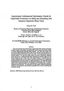
2.3 An Overview of the Approximate Dual Projective Algorithm In this section, we give a brief overview of the Approximate Dual Projective (ADP) algorithm for linear programming. For a complete description of the algorithm please see [42]. As the name implies, ADP method is an approximation to the projective algorithm of Karmarkar [40] applied to the dual. The projective algorithm has very nice stability properties, since the iterates of the projective algorithm always stay on the central trajectory [13]. The ADP method makes discrete approximations to the continuous central trajectory. Asymptotically, after a large number of iterations, the discrete approximations converge to the central trajectory. The discrete approximation consists of two steps; the objective step, and the reciprocal-estimates-improvement (REI) step. Figure 2.1 depicts the ADP method. In the gure, the optimal vertex is shown as a solid bullet at the top, and the central trajectory is shown as a double solid line. The objective step is the dual ane scaling step [1, 42] that improves the objective function. The REI step has the eect of bringing the iterate closer to the central trajectory. The name reciprocal estimates improvement comes from the fact that on the central trajectory of the dual polytope, the reciprocals of slack variables are exact primal feasible solutions up to a multiple [42]. Thus if we take a step in the dual polytope that improves the primal feasibility of the reciprocals of slacks, then this necessarily implies that the step brings the iterate closer to the central trajectory. The approach


9

Optimal Solution Objective Step Central Trajectory Reciprocal Estimates Improvement Step

Starting Solution

Figure 2.1: Pictorial View of the Approximate Dual Projective(ADP) Algorithm of improving reciprocal estimates is an interesting interpretation of the traditional way of P centering, i.e., that of minimizing the potential function ? ln si , where si is the dual slack variable. In fact, the linear systems solved by the newton-method-based minimization of the potential function and the REI step are identical. The ADP algorithm is similar to the BLCA algorithm of Todd [76], the ane scaling algorithms of Gonzaga [30],Barnes, Chopra, and Jensen [12], and many others. All these algorithms use ane scaling with centering on the primal problem. Recently, dual ane scaling algorithm with centering was studied by Hipolito [31]. Generally the ADP method consists of two phases. In Phase 1, the dual phase, the dual of the LP problem is solved; and in phase 2, a primal solution is obtained, starting with the estimates from the converged dual solution. At the end of execution of both phases, a primal-dual pair with a small relative duality gap is obtained. We now give a brief overview of the ADP method. Consider the LP problem, with upper bounds in standard primal form: (2.4)

min cT x

subject to (2.5)

Ax = b

(2.6)

0xu:


10

Here A 2 Rmn; c; x; u 2 Rn, and b 2 Rm . Introducing dual variables y and z , corresponding to 2.5 and 2.6 respectively, the dual of 2.4{2.6 becomes (2.7)

max bT y + uT z

subject to (2.8)

AT y + z c

(2.9)

z0:

De ning (2.10)

s2 = ?z

and introducing slack variables s1 in 2.8, the dual 2.7{2.9 becomes (2.11)

max bT y ? uT s2

subject to (2.12)

AT y ? s 2 + s 1 = c

(2.13)

s1 ; s2 0 :

We can now develop a variant of the dual projective algorithm for solving 2.11{2.13. The scaling matrix D is de ned in partitioned form as (2.14)

2 66 D1 D = 64

D2

3 77 75 ;

where (2.15)

D1?1 = diag (s1)

and (2.16)

D2?1 = diag (s2 ) :


11

Let y , s1 , and s2 be the ascent directions used in the algorithm. Given below are the formulas for y , s1 , and s2. The derivation of these formulas is identical to the derivation in [1] except for the treatment of upper bounds on the primal variables. The derivation of these formulas in the presence of upper bounds can be found in [41]. (2.17) y = (AD~ 2AT )?1 (b ? AD12 De2u) (2.18)s1 = ?De2 D22AT (AD~ 2 AT )?1(b ? AD12 De2u) ? De2 u (2.19)s2 = De2D12 AT (AD~ 2AT )?1(b ? AD12De2 u) ? De2 u where (2.20)De?2 = D12 + D22 (2.21) D~ 2 = D12 ? D12De2 D12 : The ADP algorithm is given below.

APPROXIMATE DUAL PROJECTIVE ALGORITHM: DUAL PHASE 1. Given an initial interior starting point y 0 , s01 , s02 and parameters , and , set the iteration counter i = 0; switch criterion = false. 2. WHILE switch criterion is false DO 2.1 // Objective function improving step. a) Compute ascent directions y , s1, and s2 using equations 2.14 to 2.21. b) // compute maximum step length permissible to keep s1 and // s2 nonnegative. i i s s 1 k = min min ? ; min ? 2m s k or zel ? z~el =z~el > set x~le = xle and z~el = zel , and update Dl ; C l and C using rank one updates. .

.

Claim 3.4.6 The complexity of step 1 is O(kn3 + km2 + m3). Proof: Because of the structure of B as vertex-edge adjacency matrix each entry of

BDl? B T can be computed by at most one subtraction depending on whether there is an edge between the two vertices that de ne the entry. Hence computing each matrix C l in step 1b can be done in O(n3 ) time. Using the same argument, we can prove that each entry of Dl? B T C l BDl? can be computed in constant time using only 4 entries in C l . All 1

1

1

other estimates are standard.

Claim 3.4.7 Each update in step 5 can be done in O(m2) time.

CHAPTER 3. QUADRATIC PROGRAMMING APPROACH

33

Proof: Since each update in step 5 is a simple rank one update, we can prove the claim

using the Sherman-Morrison-Woodbury formula.

p Claim 3.4.8 Assuming that r mk, the total number of updates done in step 5 in the r iterations between two applications of step 1 is O(r2).

Proof is the same as in [39].

Theorem 3.4.9 The average complexity of Variant-2 is O(m2:5 + k0:5mn1:5 + kn2). Proof: The average complexity of step 1 is O ((kn3 + m3 + km2)=r). The complexity of steps 3 and 4 is O(m2 + kn2 ). The average complexity of step 5 is O(rm2) (using claims 3.4.7 and 3.4.8). Choosing r to balance these terms we get the result.

Theorem 3.4.10 Assuming usage of fast matrix multiplication procedure that inverts an n n matrix in O(n2:4) time the average complexity of the procedure Variant-2 is O(m2:2 + k0:5m2 + k0:5mn1:2 + kn2 ).

3.5 Starting Point For The Algorithm In this section, we provide a good starting point for our algorithm that enables us to prove a good complexity for our approximation algorithm. The idea behind the choice of the point is outlined below. The algorithm can be shown to converge rapidly if we start at a point close to the central path. As converges to in nity the central path converges to the center of the polytope (the minimizer of the barrier function). Since our constraints are separable it is very easy to calculate this center by splitting the capacity equally between the commodities. Near the center of the polytope, the value of changes rapidly on the central path and we can show a polynomial bound on , for which our starting point is a -approximation. We can set w0 = (x; y; z) as follows: (e) denote x = (x ) xle = xse = xe = ku+ e e2E 1

ye = ? x + BT Bx e e

z = c + Qx ? AT y


34

Theorem 3.5.1 We can nd such that w0 is a approximation to the central path () at with log = O(log(?1nUD)).

Proof: As mentioned above the values of x are chosen to minimize the barrier function

(regardless of the objective function). The values of y are chosen such that zel = cle + BT Bx e ? ye = cle + x = cle + (uk(+e)1) 8l 2 K n fsg e

zes = ?ye = x ? BT Bx e e

The values of z are set by the feasibility of the dual problem. The proof of the theorem follows from the next two claims.

Claim 3.5.2 If 2nUD then (x; y; z) is primal and dual feasible. Proof: The only non-obvious thing to check is z 0. Now zel = cle + (uk(+e)1) ?D + k U+ 1 0

zes = x ? B T Bx e (ku+ 1) ? 2n k U+ 1 0 e

Claim 3.5.3 Pe2E;l2K (zel xle ? )2 nkD2U 2 + 4mU 4n2 Proof: The distance from the central path can be bounded as X X (zel xle ? )2 = (clexle )2 nkD2 U 2 e2E;l2K nfsg

X e2E

e2E;l2K nfsg

(zesxse ? )2 =

X e2E

( ? xe B T B x e ? )2

U 2 U m k + 1 2n k + 1 4mU 4n2:

The theorem now follows since we proved that for which is polynomial in ?1 ; n; d and U the chosen point is a feasible point and a approximation to the central path at .


35

3.6 Stability In this section, we will bound the precision needed in performing each arithmetic operation.

Claim 3.6.1 A vector x is the global optimum solution of X min cT x + 12 xT Qx ? i ln xi i

s. t. Ax = b x 0 if and only if there exist vectors z and y such that the following Karush-Kuhn-Tucker conditions are met:

8i xizi = i Ax = b x 0

?Qx + AT y + z ? c = 0 z 0:

Proof: Using standard primal-dual arguments. Claim 3.6.2 Let w = (x; y; z) be a approximation to the central path () at then

log zel =xle is O (log((1 + )nU )) and log xle=zel is O (log((1 + )?1 U )) for every edge e and commodity l.

Proof: Set le = xlezel 2 [(1 ? ); (1 + )]:

(3.2)

Using claim (3.6.1) we know that x is the minimizer of

E (x) ?

(3.3) s.t. 8e 2 E

X l2K

X

e2E l2K

xle = u(e):

For a given e = vw 2 E and l; j 2 K de ne

?

le ln xle

?

p(t) def = Exv (xl ) ? hl (v ) ? t 2 + Exw (xl ) ? hl (w) + t 2 ? ? + Exv (xj ) ? hj (v ) + t 2 + Exw (xj )hj (w) ? t 2 ? le ln(xle + t) ? je ln(xje ? t)


36

From the fact that x minimizes the potential function de ned in 3.3 we can deduce

? @ p ( t ) = 2 ?Exv (xl ) + Exw (xl ) + Exv (xj ) ? Exw (xj ) 0 = @t t=0 ? le x1l + je 1j xe e

Using the bounds in (3.2) we get 1 1 + + 2 ? Ex (xl ) + Ex (xl ) + Ex (xj ) + Ex (xj ) v w v w xle xje (1 + ) 1 +j + (1 2+ ) 4nU

xe Since for every e there exists j 2 K such that xje u(e)=(k + 1) 1=(k + 1) we get that for every e 2 E and l 2 K 1 (1 + )(k + 1) + 2 4(nU + D): xl (1 + ) e

The claim follows now from the facts (1 ? ) xle zel (1 + ) and xle U .

Claim 3.6.3 In each iteration, the logarithms of the condition numbers of the matrices

involved are O (log(UDn)).

Proof: Since the matrix Dl + BT B is symmetric and positive de nite we can estimate max xT (Dl + B T B)x maxe zel =xle 2(Dl + B T B) = min kxk =1 xT (Dl + B T B)x n +min kxk =1 e zel =xle 2

2

and the claim about this matrix follows from the previous claim. For the matrix

0 1?1 X ? @(Ds)?1 + Dl + B T B ?1A l2K nfsg

note that it is the sum of symmetric positive de nite matrices and hence the claim follows also for this matrix. All the other matrices that appear in the computations can be bounded in the same way.

Theorem 3.6.4 To compute a solution with b bits of precision, the computations need to be done with O (b + log(nUD)) bits of precision.

Proof: Using the theorem 3.3.2 we know that if only b bits of precision in the solution

are needed we need to continue the algorithm until log ?1 becomes O(b + log(nUD)). The theorem now follows from the previous claim.


37

There are two conditions that should be satis ed at each iteration, namely, Ax = u and z = c + Qx ? AT y . When working with in nite precision the conditions are maintain because of the de nitions of w = (x; y; z ). When working with nite precision in order to avoid accumulation of rounding errors we should calculate the following values in the end of each iteration again:

xse = u(e) ?

X

l2K nfsg

xle

z = c + Qx ? AT y The variables resulting from these corrections can be shown to obey central path conditions since the only errors are those introduced by rounding.

3.7 Finding an Exact Solution If we nd an -approximate solution then for suciently small , we can round to an exact solution using the technique described in [79]. The conditions under which the technique is guaranteed to give an exact solution is stated in the following theorem, which is proved in [79].

Theorem 3.7.1 If there exists an optimum solution to a quadratic programming problem in n variables, in which every non zero variable is at least then an 2 =n-approximate solution can be rounded to an exact optimum solution in O(n) time. To use this result we will prove the following theorem:

Theorem 3.7.2 Given a multi-commodity ow problem which has a solution, we can nd > 0 such that log ?1 = O(m log m +log UD) and such that there exists a solution in which every non zero ow is at least .

Proof: Formulate the multi-commodity ow problem as a linear programming feasibility

problem, where a variable is associated with every path between a source and a sink of a commodity. We will denote by xp the variable corresponding to the ow on the path p. The constraints are:

8p xp 0


8i k 8e 2 E

X p:p

from si to ti xp u(e)

38

xp = di

X

p:e2p

Using the theory of linear programming, we know that every linear optimization problem has a vertex solution which is de ned by a solution of a linear system which is a sub-matrix of the constraints matrix. Using Cramer's rule we can give a lower bound on a non-zero entry in the solution by giving an upper bound on the determinant of a sub-matrix of the constraints matrix. The constraints matrix is exponential in size, but it is easy to check that all the rows associated with the equalities of the type xp 0 do not contribute to the determinant. Hence every subdeterminant is bounded by the determinant of a (m + k) (m + k) matrix with entries in f0; 1g. Hence the theorem follows. Note also that for a given ow solution, we can always use the zero vectors for the dual variables (this can be proved either directly from the equations, or intuitively, by noting that the optimal value on the polytope of the objective function is also the global optimal value).

Theorem 3.7.3 An exact solution to the multi-commodity ow problem can be obtained by

computing an -approximate solution where log ?1 = O(m log m + log U + log D).

3.8 Extensions In this section, we show that our results extend to other variants like minimum cost multicommodity ow, concurrent ow and generalized multi-commodity ow.

3.8.1 Minimum Cost Multi-commodity Flow. The minimum cost multi-commodity ow instance is a multi-commodity ow instance with costs p(e) 0 on the edges e. The optimum ow is the solution to the multi-commodity P P

ow problem which minimizes the cost function P (x) = e p(e) l xle. Denote by p 2 RE the vector of costs and let P be the maximum cost. In order to nd an -approximate solution to the problem we will use our algorithm on the following objective function:

F(x) def = PUm E (x) + P (x):


39

Theorem 3.8.1 The results that we obtained for the multi-commodity ow problem (com-

plexity, starting point, stability and exact solution) also hold for the minimum cost multicommodity ow problem with additional log of the ratio between biggest and smallest cost in the number of iterations.

To prove the theorem we will state several claims that will show how we can use the results for the multi-commodity case for the case of ow with costs.

Claim 3.8.2 Assume that p is the minimum cost of a solution to the multi-commodity ow problem and F is the optimum value of F . Also, assume that for a given pre-multi- ow x, we have F (x) F + , then

E (x) 2 P (x) p + :

Proof: Let x be the minimizer of F and x~ the minimum cost ow, then F(x) F(~x) = P (~x) = p : Thus

P (x) F (x) F (x ) + p + : Using the same inequalities hence

PUm E (x) p + :

p 2: + PUm E (x) PUm

Claim 3.8.3 The complexity of computing a single iteration for the minimum cost multicommodity ow problem is the same as that for the feasibility problem.

Proof: Since the only change from the original problem was changing the linear part of

the objective function the algorithm stays exactly the same. The linear part does not aect the computation of a single iteration.


40

Claim 3.8.4 We can nd a starting point w = (x; y; z) and such that w is a approximation to the central path () at with log = O(log(?1 nUDP?1 )). Proof: Following the same idea as in section 3.5 we will choose the following starting point for a given :

(e) xle = xse = xe = ku+ 1

denote x = (xe )e2E

BT Bx ye = ? x + PUm e e PUm Qx ? AT y c + p + z = PUm Calculating the z 's explicitly gives (note that slack variables are not multiplied by the prices):

PUm T PUm l l zel = PUm ce + p(e) + B Bx e ? ye = ce + p(e) + xe l + p(e) + (k + 1) 8l 2 K n fsg = PUm c e u(e) BT Bx zes = ?ye = x ? PUm e e In order to check the feasibility of the starting point we need to check if z > 0. The z 's can

be estimated as (compare to claim 3.5.2) (k + 1) DPUm (k + 1) 8l 2 K n fsg l zel = PUm ce + p(e) + u(e) ? + U BT Bx (k + 1) ? PUm 2n U : zes = x ? PUm e U k+1 e Hence if max(?1 DPU 2 m; U 3Pm?1 2n) then (x; y; z ) is primal and dual feasible. Estimating the distance of w from the central path at gives (compare to claim 3.5.3)

X

e2E;l2K nfsg

X e2E

(zel xle ? )2

(zesxse ? )2 =

=

X e2E

X

e2E;l2K nfsg

2 PUm l l xe ce + p(e) 2m3U 3P 2D2 ?2

T 2 ( ? xe PUm B Bx e ? )

U 2 4m3 U 6n2 P 2?2 m k U+ 1 PUm 2 n k+1 Hence we can nd a feasible starting point which is a approximation to the central path at where is a polynomial in n; U; D; P and ?1 .


41

Claim 3.8.5 The stability results proved for the multi-commodity ow problem hold for the

minimum cost multi-commodity ow problem.

Proof: Following the same proof as in section 3.6 proves the claim. An additional term of log P should be added to the number of bits to be used.

3.8.2 The Concurrent Flow Problem. A concurrent ow problem involves nding the minimum factor such that the demands can be satis ed with capacities scaled to u(e). In order to nd an -approximate solution to the concurrent ow problem we will de ne for > 0 the following objective function

G(x; t) def = E (x) ? t We will nd an approximate solution to the problem by minimizing G(x; t) subject to

8e 2 E

X

l2K

xle + tu(e) = u(e) t 0 xle 0:

To ensure that a solution exists we will multiply each capacity by kD.

Theorem 3.8.6 The results that we obtained for the multi-commodity ow problem (com-

plexity, starting point, stability and exact solution) apply to the concurrent multi-commodity

ow problem as well.

To prove the theorem we will state and prove several claims that will show how to use the same methods obtained for the multi-commodity ow problem to the concurrent ow problem.

Claim 3.8.7 Assume that 1. Suppose that ~t is the optimal value of the concurrent ow

problem and that G is the optimal value of G subject to the constraints. Assume that for a given pre- ow x and parameter t we have G (x; t) G + 2 , then

t ~t ? E (x) 2

Proof: Let (~x; ~t) be the solution for the concurrent ow problem. Then G G (~x; ~t) = ?t~


42

hence

?t G(x; t) G + 2 ?t~ + 2 which implies the rst inequality. In addition to that

E (x) = G(x; t) + t G + 2 + t Note that always G 0, t 1, 1 , hence

E (x) 2

Remark: Note that since we scaled the capacities by kD to ensure the existence of

a solution, an -approximation to our problem is an kD approximation to the original concurrent ow problem.

Claim 3.8.8 The asymptotic complexity of one iteration in optimizing G is the same as in the multi-commodity ow problem.

Proof: The algorithms described in section 3.4 are can be seen as solving the following

linear system:

1 10 1 0 0 XZe ? ^ e x Z 0 X CC CC BB CC B B B B = CA B C B C B 0 @ A 0T 0 A @ y A @ 0 z ?Q A I

In the concurrent- ow problem we have two additional variables t and zt and the matrix to solve is the following:

0 BB Z BB 0 BB A BB @ ?Q

10

1 0

1

0 X 0 0 CC BB x CC BB XZe ? ^e CC 0 0 zt t C B y C B 0 CC CC BB CC BB CC 0 0 u 0 C B z C = B 0 C B B C CC AT I 0 0 C 0 A B@ t CA B@ A 0 uT 0 0 1 zt 0 Hence the linear system for the concurrent ow case is the same as the multi-commodity ow case, except a constant number of rank one updates. Using the Sherman-Morrison formula, it then follows that the complexity of solving the linear system is a constant multiple of that for the multi-commodity ow case.


43

Claim 3.8.9 We can nd a starting point w = (x; y; z; t) and such that w is a approximation to the central path () at with log = O(log(?1 nUD?1 )). Proof: As in section 3.5 we will use as a starting point the point that minimizes the

barrier function regardless of the objective function. By dierentiating the barrier function we get that the starting primal-dual point (x; y; z; t) for a given is: t = m(k +11) + 1 (e) xle = xse = xe = (1 ? t) ku+ 1

denote x = (xe )e2E

ye = ? x + BT Bx e e

k + 1) 8l 2 K n fsg zel = cle + BT Bx e ? ye = cle + x = cle + u(e()(1 ? t) e

zes = ?ye = x ? BT Bx e e

zt = ? ?

X e2E

u(e)ye = ? +

X u(e) T x ? B Bx e

e2E

e

1 ? B T B x = ? + (m(k + 1) + 1) ? B T B x = ? + m k1 + e e ?t To ensure that the point (x; y; z; t) is primal-dual feasible we have to check that z > 0. Estimating z can be done by (compare to claim 3.5.2): k + 1) ?D + (k + 1) zel = cle + u(e()(1 ? t) U

zes = x ? B T Bx e (kU+ 1) ? 2n k U+ 1 e

zt = ? + (m(k + 1) + 1) ? B T Bx e ?1 + (m(k + 1) + 1) ? 2n k U+ 1

Hence if max(UD; 2U 2n) then (x; y; z; t) is primal and dual feasible. To bound the distance from the central path we can calculate (compare to claim 3.5.3):

X

e2E;l2K nfsg

(zel xle ? )2 =

X

e2E;l2K nfsg

(clexle )2 nkD2 U 2


X e2E

(zesxse ? )2 =

X e2E

44

( ? xe B T B x e ? )2

U 2 U m k + 1 2n k + 1 4mU 4n2 (tzt ? )2 = (?t + t(m(k + 1) + 1) ? t B T B x e ? )2 2 5n2U 2 = (?t ? t B T B x )2 + 2n U e

k+1

Hence for polynomial in n; D; U and we know that (x; y; z; t) is a approximation to the central path at .

Claim 3.8.10 We can nd an approximate solution to the concurrent ow problem with the same asymptotic complexity as in the multi-commodity ow problem.

Proof: Given > 0, in order to nd an approximation to the concurrent ow problem we will nd the approximate optimal of G (). Claim 3.8.7 proves that this will give an approx-

imate solution to the concurrent ow problem. Combining claim 3.8.9, theorem 3.3.1 and theorem 3.3.2 (adjusted to G instead of the original quadratic objective function) assures p us that an approximate solution will be calculated in O( mk log(nDU?1 )) iterations. Claim 3.8.8 assures us that the complexity of each iteration is the same.

Claim 3.8.11 We can nd an exact solution to the concurrent ow problem with the same asymptotic complexity as the multi-commodity ow problem.

Proof: Following the same technique as in the multi-commodity case, we will show that

the number of bits needed to compute an exact solution is O(m log m + log UD) which is sucient to prove the claim. To bound the number of bits needed to describe an exact solution we will follow the same proof as in section 3.7, adjusted to the concurrent ow problem. We will associate a variable with every path from a source and a sink of a commodity. In addition slack variables s(e), and a variable t will be de ned. The linear constraints de ned for each edge will be:

8e 2 E;

X

p:e2p

xp + s(e) + tu(e) u(e)

Estimating the solution in the same way, we have to bound the determinant of an m + k m + k matrix in which all entries are 0 or 1, except possibly the column containing the capacities. Hence the claim follows.


45

3.8.3 The Generalized Flow Problem. For the de nition of the generalized ow problem see [25]. In this problem, ows moving on edges have dierent gains or losses. To solve the generalized multi-commodity ow problem using our algorithm, all we have to change are the entries in B which instead of being 0 and 1, will now depend on the gain/loss factor on the edges. Let be the ratio between the biggest and smallest generalized ow coecients. The next two theorems can be easily veri ed:

Theorem 3.8.12 Each iteration of our algorithm, as applied to the generalized multicommodity ow problem has the same complexity as for the original multi-commodity ow problem. However, for nding the exact solution there is an additional O(log ) factor in the number of iterations and for nding an approximate solution there is an additional factor of n log .

Proof: Since complexity proofs used only the sparseness of B and not the fact that all

entries are either 0 or 1, the complexity of a single iteration remains the same in the generalized ow problem. In the estimation of the starting point, will depend polynomially on , adding a log factor to the running time. Also, in converting a pre- ow to a ow, we can gain or lose as much as n factor. Hence, to satisfy 1 ? fraction of all the demands, we may need more accurate solutions, giving an additional term of n log in the number of iterations.

Theorem 3.8.13 We can solve the single commodity generalized ow problem without using fast matrix multiplication in O (n2 m1:5 log(nUD )).

Proof: We will use the conjugate gradient variant to compute each iteration and hence the

complexity of each iteration is O(mn). To estimate the convergence criterion for rounding to the exact solution, we have to bound the largest sub-determinant of the matrix,

0 1 Q A @ A: A 0

In our case, the matrix is

1 0 T B B 0 I C BB B@ 0 0 I CCA : I

I 0


46

Since the log of the biggest subdeterminant of B T B is O(n log n ) and the number of variables is 2m the overall complexity of our algorithm is O(mn m0:5 (n log n + log DU )) and the theorem follows.

Chapter 4

Distributed Algorithm for Multi-commodity Flow 4.1 Introduction In this chapter1 , we present a simple and fast distributed approximation algorithm for a variant of the minimum-cost concurrent multi-commodity ow problem. One can ask the question, why we need an approximation algorithm, when the problem can be written as a linear program which can be solved exactly using interior point methods. Unfortunately, the fact that the number of variables is large causes these methods to generate rather slow (large computational complexity) algorithms. In particular, as seen in Chapter 3, the fastest interior-point min-cost multi-commodity ow algorithm [34, 39, 77, 78] relies on fast matrix multiplication subroutine and takes O(k3:5n3 m:5 log(nDU )) time for the multi-commodity

ow problem with integer demands and at least O(k2:5nm1:5 log(n?1 DU )) time to nd an approximate solution, where D is the largest demand, and U is the largest edge capacity. Moreover, since this algorithm involves repeated matrix multiplications, it does not seem appropriate for ecient implementation in the distributed setting. Signi cantly better running times were achieved by approximation algorithms. In particular, if there exists a feasible solution, then the algorithm due to Leighton, Makedon, Plotkin, Stein, Tardos, and Tragoudas [49] will produce an -approximation to the feasible

ow in O (k2mn?2 ) time. A ow that both satis es at least (1 ? ) fraction of each demand and whose cost is within (1 + ) of the optimum can be obtained by the algorithm due to 1

This chapter represents joint work with Omri Palmon and Serge Plotkin [35].

47

CHAPTER 4. DISTRIBUTED ALGORITHM

48

Plotkin, Shmoys and Tardos [67] in O (k2 m2?2 log C ) time, where C is the maximum edge cost. The running times of these algorithms can be improved by a factor of k by use of randomization. Radzik [68] showed a deterministic technique to improve by a factor of k, the complexity of the Leighton et al. algorithm. Later Karger and Plotkin [34] modi ed the algorithm in [67], to give a deterministic algorithm for the minimum cost multi-commodity

ow which has an improved complexity of O (kmn?3 log C ). All these algorithms are based on repeated computations of minimum-cost ows or shortest paths, and hence are not very easy to implement in a distributed setting. (Especially in networks with dynamic topology.) The best performance one can hope to achieve by implementing the algorithm in [67], in a static network is O (kmn?2 log C ) rounds. This signi cantly exceeds the number of rounds of the algorithm presented in this chapter for large k and constant ; . If there exists a feasible ow, i.e. ow that satis es all the demands, then in O (m2?2 ) communication rounds, our algorithm nds a ow that satis es at least (1 ? )-fraction of each demand, where m is the number of edges in the network.2 If there exists a feasible

ow of cost B , then our algorithm nds a ow that satis es (1 ? ) fraction of the demands and whose cost is below (1 + )B in O (m2?2 ?2 log(CU )) rounds, where C and U are maximum edge cost and maximum edge capacity, respectively. A communication round consists of each processor performing a computation on its local data and sending the results to all of its neighbors. Our algorithm is local in a sense that it does not depend on any global computations like shortest paths or min-cost ow, that were the main subroutines of the previously known ecient combinatorial multi-commodity

ow algorithms [47, 49, 67]. The only previously known local approximate concurrent ow algorithm, due to Awerbuch and Leighton [8, 9], does not address the min-cost problem. The main advantages of a \local" algorithm is ease of implementation in a distributed system where centralized control is either infeasible or very expensive. Moreover, our algorithm is resilient to failures: an edge failure (or, as a matter of fact, and change in the network topology) that does not make the problem infeasible, can delay the convergence of the algorithm by at most the number of rounds stated above. The only two nodes needed to be noti ed about the failure are the nodes adjacent to the failed edge. This makes it unnecessary to run the complicated and costly \global reset" algorithms [2] after every failure/reappearance of an edge. Another interesting property of our algorithm is that it can be modi ed to run forever, maintaining an approximate solution to the ow, automatically 2

We say that f (n) = O (g(n) if f (n) = O(g(n) log n) for some constant k. k


49

adjusting it after every edge failure or demand change. The algorithm presented in this chapter is very simple. The idea is to maintain a pre ow, which is ow that obeys capacity constraints but does not obey ow-conservation constraints. We refer to the dierence between the ow into a node and the ow out of the node as the excess at this node. The algorithm starts with zero ow, which is a valid pre ow. Each iteration consists of two phases. In the rst phase, each node distributes its excess among its adjacent edges. Then, independently for each edge, the ow through the edge is updated in a way that reduces a certain non-linear function of the excesses assigned to this edge. Intuitively, this operation \spreads" the excesses throughout the graph, eventually obtaining a solution with very small excesses. Our algorithm is in some sense similar to the one in [8]. There are two main dierences that allowed us to get improved performance. First, we use a dierent local optimization criteria. Our criteria can be viewed as an adaptation to the excess-minimization context of the exponential \length function", introduced by Shahrokhi and Matula [71]. Second, we use pre ow instead of explicitly maintaining queues. Roughly speaking, if one interprets

ow as the \amount of ow in unit time", then the fact that a node has excess implies that each time unit there is more ow coming in than going out. The algorithm in [8] explicitly maintains the number of ow units queued at each node and tries to minimize the size of these queues. Instead, our algorithm minimizes the excess, which corresponds to the rate of growth of the queues.

4.2 Preliminaries and De nitions As de ned in previous chapters, an instance of the multi-commodity ow problem consists of an undirected graph G = (V; E ), a non-negative capacity u(vw) for every edge vw 2 E , and a speci cation of k commodities, numbered 1 through k, where the speci cation for commodity i consists of a source-sink pair si ; ti 2 V and a non-negative demand di. Also, for notational convenience, we arbitrarily direct each edge. If there is an edge directed from v to w, this edge is unique by assumption, and we denote it by vw. A multi-commodity ow f consists of a function fi (vw) on the edges of G for every commodity i, which represents the ow of commodity i on edge vw. If the ow of commodity i on edge vw is oriented in the same direction as edge vw, then fi(vw) will be positive, otherwise it will be negative. The signs only serve to indicate the direction of the ows.


50

Given ow fi (vw), the excess Exi (f; v ) of commodity i at node v is de ned by: Exi (f; v ) def = di (v ) ?

X w:vw2E

fi (vw);

where di(si ) = di, di (ti ) = ?ti and di(v ) = 0 otherwise. This de nition of excess is slightly dierent from the earlier de nition given in Chapter 3. A ow where all excesses are zero is said to satisfy the conservation constraints. A ow P satis es capacity constraints if i jfi(vw)j u(vw) for all edges vw. A ow that satis es both the capacity and the conservation constraints is feasible. During the description of our algorithm it will be convenient to work with pre ow, which is a ow that satis es capacity constraints but does not necessarily satisfy the conservation constraints. An approximation to the multi-commodity ow feasibility problem is a feasible ow that satis es at least (1 ? ) fraction of the demands for each commodity.

4.3 The Flow Without Costs In this section we present the distributed multi-commodity ow algorithm. If a feasible solution satisfying all the demands exists, the algorithm will produce a ow that satis es at least (1 ? ) fraction of each demand.

The Algorithm The algorithm starts with zero ow, which is a valid pre ow. The algorithm maintains for every node pair v; w such that vw 2 E or wv 2 E , commodity i, and edge vw 2 E an excess Exi (f; vw).3 Excess of commodity i at node v is the sum

of Exi (f; vw) for all w. Each iteration consists of two phases. In the rst phase, each node recomputes Exi (f; vw), eectively distributing its excess among its edges. Then, independently for each edge, the ow through the edge is updated in a way that reduces the potential function de ned below. Intuitively, this operation \spreads" the excesses throughout the graph, eventually obtaining a solution with very small remaining excesses. Given a ow f , we de ne the following potential function:

(4.1) 3

k XX

def

(f ) =

vw2E i=1

Ex (f; wv) Ex (f; vw) i + exp i ; exp di

Note that, in general, Ex (f; vw) = Ex (f; wv). i

6

i

di


51

where

def = 4?1m log(mk): The algorithm starts from the zero ow and proceeds in iterations, where each iteration consists of two phases. The rst phase computes the excess Exi (f; v ) at each node and distributes it equally among the edges incident to this node by setting Exi(f; vw) = Exi (f; v )= (v ), where (v ) is the degree of v . The second phase calculates the ow update fi (vw) on each edge vw for each commodity i where the goal is to minimize the potential function (f ). In fact, since this function can be written as a sum of functions where each one depends on the ow on a single edge, the algorithm minimizes the following function independently for each edge vw: k X

(4.2)

i=1

Ex (f; wv) + f (vw) Ex (f; vw) ? f (vw) i i i + exp i : exp di

di

In order to ensure convergence to feasible ow, the minimization is done under the following constraints: k X i=1

jfi(vw) + fi(vw)j u(vw) jfi(vw) + fi(vw)j di

The new ow is computed by setting fi (vw) = fi (vw) + fi(vw). In the rest of this section we will assume that the minimization is executed as described above. In fact, one can minimize a much simpler expression, thus improving the complexity of each iteration. We will address this issue in Section 4.4.

Analysis of the algorithm We will show that existence of a feasible solution that satis es

all of the demands implies that each iteration reduces the potential function. We will concentrate on proving the reduction due to the second phase in each iteration, since the rst phase can not increase the potential function. The following theorem shows that suciently small value of (f ) implies that the sum of the excesses of any commodity does not exceed an -fraction of the demand of this commodity. Note that such a pre ow can be easily converted into a ow that satis es (1 ? )-fraction of each demand.

Theorem 4.3.1 If the value of the potential function (f ) exp ? m then for each P commodity i, we have jEx (f; v )j d . v

i

i


52

Theorem 4.3.2 For each iteration (f + f ) (f ) : Furthermore, if there exists a feasible solution to the problem then in each iteration ! log2 (mkf ) : (f + f ) (f ) 1 ? 162

Proof: As we have noted above, the rst phase of each iteration can not increase the

potential function. Obviously, the second phase can not increase the potential function value. It remains to prove that the decrease due to the second phase is large. Let f denote a feasible solution that satis es all of the demands such that jf (vw)j di for every commodity i and edge vw. Let f~ def = f ? f . Observe that ow update de ned by f~ for any 2 [0; ?1] satis es the optimization constraints. Hence the reduction in the potential function can be bounded by computing the eect of updating the current ow by f~. We will use the fact that ex+t ex + tex + t2 ex for jtj 1. Thus, if f~i (vw) di for all i and vw, we have: (4.3) f + f~ (4.4)

k X X i=1 vw2E

~i (vw) ! ~i(vw) ! Ex ( f; vw ) ? f Ex ( f; wv ) + f i i exp + exp d d i

i

(f ) Exi(f; wv) k X ~i (vw) Exi (f; vw) X f (4.5) ? exp d ? d exp d i i i i=1 vw2E ! 2 k X ~ X (4.6) + 22 fi (dvw) exp Exi (df; vw) + exp Exi(df; wv) : i i i i=1 vw2E

We will evaluate each one of the terms in the above expression separately. To evaluate (4.5) we decompose f~ into cycles and paths from positive to negative excesses. Notice that the cycles do not aect the value of (4.5). Moreover, each ow path of value F that starts with edge vv 0 and ends with u0 u, contributes Exi(f; vv0) Exi(f; uu0) F exp ? exp :

di

Hence, (4.5) is equal to:

di

(f ) X X Exi(f; vw) Exi(f; vw) exp (f ) log ; i vw2E

di

di

mk


53

P

where the inequality follows from the fact that the sum has mk terms and yi log yi is convex. To evaluate expression (4.6) we use the fact that f~i (vw) 2di and thus

!

~i (vw) 2 Exi(f; vw) f 2 2 exp 422 (f ) : d d i i vw2E

XX i

Combining our bounds on (4.5) and (4.6) we get from (4.3) that for ?1 : f + f~ (f ) ? (f ) log (f ) + 4 22 (f ) : Thus taking (f ) = log8km 2 we get

mk

"

2 (f )

#

log f + f~ (f ) 1 ? 16mk : 2 This completes the proof of the theorem. Remark: Note that the way we proved the decrease in the potential function is by expressing a lower bound on this decrease as a sum of quadratic functions in f and then showing that there exists a ow that achieves a large decrease. We will use this fact in Section 4.5, where we present an ecient implementation of each iteration.

Theorem 4.3.3 After O(m2?2 log mk) iterations, we have Pv jExi(f; v)j di for each commodity i.

Proof: Theorem 4.3.2 implies that as long as (f ) 2m2k2, the value of the potential

function is halved in O(2= log2 (f )). Thus, the number of iterations until the potential function falls to 2m2k2 is bounded by O (2 = log(2m2k2 )) = O(m2?2 log mk). The claim follows by substituting the value of into the claim of Theorem 4.3.1.

4.4 Flow With Costs In this section, we show how to modify the algorithm described in Section 4.3 to approximately solve the minimum cost multi-commodity ow problem. More precisely, we consider the problem where every edge vw has an associated cost c(vw), and the goal is to


54

nd a ow f that satis es at least a (1 ? ) fraction of each demand and whose cost P jf (vw)jc(vw) (1 + )B, where B is a given budget and > 0 is some given parami;vw i eter. In this section we will assume that B is given and that there exists a feasible ow of cost at most B that satis es all the demands. Note that by doing bisection search, one can easily extend our approximation algorithm to the case where B is unknown in advance. Details will appear in the full paper. In order to take the costs into account, we will use the following potential function, which is a modi cation of the function used in the previous section. Ex (f; wv) Ex (f; vw) k def X X i + exp i (f ) = exp

di XX

+ (1 + )B ci(vw)jfi(vw)j i vw2E vw2E i=1

di

where = m2 k2e4= = and = m log . To simplify notation, we will use 1 to denote the rst term and 2 to denote the second. Also, we will write instead of (f ) where it will not cause confusion. Observe that we can express (f ) as a sum of terms such that each term depends only on the ow on a single edge and is independent of the ows on the other edges. Thus, the distributed algorithm presented in Section 4.3 can be based on (f ) instead of the potential function given by (4.1). In other words, the only dierence will be the minimization step, which will update the ow on each edge in order to minimize the corresponding term in (f ) instead of the corresponding term in (4.1). As before, it is easy to see that the algorithm ensures that does not increase. Roughly speaking, our analysis consists of two parts. First we show that a suciently small value of (f ) implies that we have good approximation to the MFCB problem. Then we prove that (f ) decreases suciently fast.

Theorem 4.4.1 If pre ow f obeys capacity constraints and (f ) (1+ ), then the cost of f is at most (1 + 3 )B and the total excess of commodity i is bounded by di .

Proof: We observe that c(f ) m2k2 implies that (f ) m2k2 and hence the ow is -approximate. Moreover we also have

X X c (e)f (e) m2 k2 B i e2E i i

CHAPTER 4. DISTRIBUTED ALGORITHM and hence

XX i e2E

55

ci(e)fi(e) B(1 + ):

Observe that using the standard technique of decomposing pre ow into paths from sources to sinks, from positive to negative excesses, and into cycles, a pre ow that satis es the condition of the above theorem can be easily transformed into a ow of cost at most (1+ )B that satis es (1 ? ) fraction of each demand. This transformation is done dierently in the sequential and distributed setting and we defer the details to the full paper.

Theorem 4.4.2 The algorithm that minimizes the potential function (f ) solves MCFB

problem in O( m log2 (mk ?1 ) log (mCU )) iterations where C is the maximum cost and U is the maximum capacity associated with any edge in the graph. 2

2 2

Proof: Let f denote the optimum ow of cost at most B that satis es all the demands.

Like in the proof of Theorem 4.3.2, we will use the fact that the decrease in the total potential function at each iteration is at least as large as the decrease obtained by setting the new ow to be (1 ? )f + f . Let f = (f ? f ). Then, for 1=, the decrease in the total potential function is at least: 1 ? 4 22 (f ) + (f ) ? : (4.7) (f ) ? (f + f ) 1(f ) log mk 1 2 (1 + ) We will distinguish three cases, according to the relative values of 1 and 2 . First 4= , we get consider the case where 1 =2 and 2 1 . Using the fact that log mk that for = log8mk 2 1

1

the decrease is bounded by:

log2 mk 322 : The number of iterations of this type is at least O(2 = log(mk)). The second type of iteration occurs when 1 =2 and 2 1 . Using the same value of as above, the decrease per iteration can be bounded in this case by (=2). Since in this case O( mCU ), the number of such iterations is bounded by O(2 log(mCU )). The third type of iteration occurs when 1 =2. We will bound the number of such iterations for 2 [(1 + ) ; (1 + 2 ) ] for . When is in this range, then 1


56

2 (1 + =2) . Observe that the rst term in expression (4.7) is always nonnegative. For 1, since 2 ? =(1 + ) 2=3 by choosing = 8 2 we see that the decrease in the potential function is at least ( 2=(2 )). Hence, the number of iterations of this type for 2 [(1 + ) ; (1 + 2 ) ] is bounded by O(2 = ). Thus, the total number of such iterations for the range 2 [(1 + ) ; 2 ] is bounded by O(2). For the case where 1 =2 and 2 , choice of = 1=(82) implies that the decrease is at least (2 ), and hence the total number of such iterations is bounded by O(2 log(mCU )). Observe that if we are not in any of the types of iterations addressed above, then (1+ ) . Since monotonically decreases, the claim of the theorem follows by summing up the bound on the number of iterations of each type and applying Theorem 4.4.1.

4.5 Implementation of a single iteration The previous sections described the algorithms in terms of iterations, where the main part of each iteration is minimization of a set of independent functions of ow, one for each edge. In this section we will address the question of how to perform this minimization eciently. The main idea is to minimize a quadratic approximation to the potential function instead of the function itself. The proofs of Theorems 4.3.2 and 4.4.2 rely on the fact that the decrease in as a function of the ow update f , can be bounded by a sum of independent quadratic functions in f (one per edge), as long as the following constraints are satis ed for every commodity i and edge vw:

jfi(vw)j di= (4.8) jfi (vw) + fi (vw)j di X jfi(vw) + fi(vw)j u(vw): i

Moreover, these proofs show that there exists a f that satis es the above constraints and for which the value of the sum of these quadratic functions is suciently large. Hence, instead of minimizing the potential function itself, we can achieve at least as large a decrease by maximizing these quadratic functions over the region de ned by (4.8).


57

The advantage of working with the quadratic approximation is that it is relatively easier to optimize than the original potential function that includes exponentials. Observe that the quadratic functions that we need to maximize are concave. The quadratic optimization can be done in O(k log k) time per edge.

Chapter 5

Approximate Algorithm for Min-cost Multi-commodity Flow 5.1 Introduction Since multi-commodity ow approaches based on interior point methods for linear programming lead to high asymptotic bounds on running time, recent emphasis was on designing fast combinatorial approximation algorithms. If there exists a ow of cost B that satis es all the demands, the goal of an (; )-approximation algorithm is to nd a ow of cost at most (1 + )B that satis es (1 ? ) fraction of each demand. Approximation algorithms for various variants of multi-commodity ow can be divided according to whether they are based on relaxing the capacity [70, 47, 49, 67] or conservation constraints [8, 9]. In particular, the algorithm in [67] is based on relaxing the capacity and budget constraints. In other words, the algorithm starts with a ow that satis es the demands but does not satisfy either the capacity or budget constraints. It repeatedly reroutes commodities in order to keep demands satis ed while reducing the amount by which the current ow over ows the capacities or overspends the budget. Awerbuch and Leighton [8, 9] proposed several algorithms for multi-commodity ow without costs that are based on relaxing the conservation constraints. More precisely, these algorithms do not try to maintain a ow that satis es all of the demands. Instead, they maintain a pre ow like in the single commodity ow algorithms of Goldberg and Tarjan [26, 27]. These algorithms repeatedly adjust the pre ow on an edge-by-edge basis, with the goal of maintaining capacity constraints while making pre ow closer to a ow. 58

CHAPTER 5. APPROXIMATION ALGORITHM

59

Though the algorithms in [8, 9] have very good complexity, the main problem of extending them to the min-cost case is the fact that these algorithms are based on minimizing (at each step) a function that de nes the penalties for not satisfying the conservation constraints. The reason these algorithms are fast is that this function is separable, i.e. it is a sum of non-linear terms where each term depends on a single edge, and thus this function can be minimized on an edge-by-edge basis. A natural extension of this approach to the min-cost case is to introduce an additional penalty term that depends on the cost of the current pre ow. Unfortunately, the resulting function is non-separable since this term has to be non-linear for the technique to work. This, in turn, leads to an algorithm that has to perform a very slow global optimization at each step. In fact, this optimization does not seem to be much easier than solving the original problem. We saw in Chapter 4, one way of overcoming this problem. This gave us an algorithm which also has the nice property of being distributed. If we do not need the algorithm to be distributed, we can extend some of the ideas developed there to give a faster approximation algorithm. The main result of this chapter1 is an O (kmn2 log(CU )) deterministic approximation algorithm2 , where C and U denote the maximum cost and the maximum capacity, respectively; the constant in the big-O depends on ?1 and ?1. Our algorithm combines ideas from the feasibility multi-commodity algorithm of Awerbuch and Leighton [9] and the mincost ow algorithm described in chapter 4. As in [9], we relax the conservation constraints. In addition, we relax the budget constraint. Our algorithm maintains a pre ow that always satis es capacity constraints; the pre ow is gradually adjusted through local perturbations in order to make it as cheap and as close to ow as possible. The main innovation lies in the pair of two functions { one separable (can be minimized on an edge-by-edge basis) and one not that are used to guide the ow adjustment at each step. Essentially, the ow adjustment is guided by the separable function that is rede ned at each step, while the progress is measured by the other function, which is non-separable. There are several important dierences between our algorithm and the algorithms of Awerbuch and Leighton in [8, 9] that allow us to treat the min-cost case. Their algorithms explicitly maintain the number of ow units queued at each node and try to minimize the size of the queues by moving ow units from one queue to another. In contrast, our algorithm is based on maintaining the pre ow and the corresponding excess at each node. 1 2

This chapter represents joint work with Omri Palmon and Serge Plotkin [36]. We say that f (n) = O (g(n)) if f (n) = O(g(n) log n) for constant c. c


60

Use of pre ow instead of explicit queues required development of dierent techniques to prove the convergence. Our techniques are based on trying, at each step, to minimize a certain separable function that can be computed on an edge-by-edge basis, while measuring the progress by another, non-separable, function. We believe that these techniques might be useful for analyzing future pre ow-based multi-commodity ow algorithms. Our algorithm can be viewed as a generalization of the algorithm in [9] to the min-cost case, and as such preserves some of the advantages of that algorithm. In particular, the edge-by-edge adjustment of the ow, done by our algorithm, is inherently parallel. The mincost multi-commodity ow algorithm in [67] is based on repeated computation of shortest paths. Although this computation can be done in NC, it requires n3 processors, making it impractical. For the case where a linear number of processors is available (one for each variable, i.e. commodity-edge pair), the algorithm in [67] runs in O (kmn log CU ) time for constant and . In contrast, our algorithm runs in O (mn) time. We believe that the inherent parallelism in our algorithm, combined with locality of reference, will lead to ecient implementation on modern superscalar computers. Section 5.2 presents the continuous version of the algorithm and proves fast convergence assuming that at each iteration the algorithm computes an exact minimization of a quadratic function for each edge. In Section 5.3 we show how to reduce the amortized time per iteration by using a rounding scheme that allows us to compute approximate minimization at each iteration. Section 5.4 presents a proof that this rounding does not increase the total number of iterations.

5.2 Continuous algorithm In this section we present the (slow) \continuous" version of the min-cost multi-commodity

ow algorithm. The improvement in running time due to rounding is addressed in the next section. If a feasible solution of cost B=(1 + ) satisfying all the demands exists, the algorithm produces an (O(); O( ))-pre ow. We present here the algorithm for directed case; the undirected case can be treated similarly. We assume without loss of generality that the minimum node degree is 2mn .


61

5.2.1 The Algorithm The algorithm starts with zero ow, which is a valid pre ow. For every node pair v; w such that vw 2 E or wv 2 E and commodity i, it maintains an excess Exi(f; vw).3 The excesses Exi (f; vw) are maintained such that for every commodity i at node v , the excess Exi (f; v ) of the commodity at that node is equal to the sum of Exi (f; vw) for all w such that vw 2 E or wv 2 E . Given a ow f , we de ne the following potential function: = 1 + 2~ 1 where 1 =

X i;vw2E or wv2E

exp Exi (df; vw) ;

1X

2 = B

e2E

i

c(e)f (e):

We use di to denote the original demand of commodity i. ~ 1 is the current approximation to the current value of 1 and should satisfy: (1 + )?11 ~ 1 (1 + )1:

(5.1)

As we show below, the best performance is achieved for

= 8?1 m log(2mk);

= =(2m): Roughly speaking, 1 measures how close the current pre ow is to a ow and 2 measures how close the cost of the current ow is to the budget B . Unfortunately, it is not clear how to use to directly measure the progress of the algorithm, since it is rede ned each time 1 changes by more than a constant factor. Instead, we de ne another potential function: 1 = log 2mk + 1 + 2: The algorithm starts from the zero ow and proceeds in phases. In the beginning of a phase, we choose = 16m n 0 , where 0 is the value of potential function in the beginning of the phase. Each phase proceeds in iterations, where each iteration consists of the 2

3

Note that, in general, Ex (f; vw) = Ex (f; wv). i

6

i


62

following steps: Algorithm 1: (single iteration) 1. Add capacity u(vw) to each edge vw 2 E . Change demand of each commodity i: di = di + di , where di is the original demand of commodity i. Update the value of excesses accordingly.

2. Find the increment f in the ow vector f that minimizes under the constraint P 0 fi (vw) di and fi (vw) is less then the available capacity. Update f = f + f . 3. Recompute new excess Exi (f; v ) at each node and distribute it equally among the edges incident to this node by setting Exi (f; vw) = Exi (f; v )= (v ), where (v ) is the degree of v . 4. Update the current value of ~ 1, if necessary. A phase is terminated either after 1= iterations or when the value of falls below 0 =2. In the end of a phase, we scale down all the ows, the demands, and the capacities (and hence all the excesses) by a factor of 1 + r , where r is the number of iterations in this phase. Note that in the end of each phase the capacities and the demands are equal to the original capacities and the demands. Moreover, since we scale ows and capacities by the same factor, the pre ow in the end of each phase satis es the original capacity constraints. The second step is the heart of the algorithm. Since function is separable, i.e. can be written as a sum of functions where each one depends on the ow on a single edge, the algorithm computes change in ow f by minimizing the following function independently for each edge vw 2 E : k X i=1

fi (vw) exp Exi (f; vw) ? fi (vw) + exp Exi (f; wv) + di

di

+ B ~ 1 c(vw)fi (vw):

5.2.2 Bounding number of phases In this section we show a bound on the number of phases of Algorithm 1. Initially, we assume that each phase is executed exactly as stated above, i.e. the minimization in step 2


63

and the excess rebalancing at step 3 are computed exactly. First we show that suciently small value of implies that the current ow is close to optimum.

Lemma 5.2.1 If (1 + ) , then the current pre ow is (2; 3)-optimum. Proof: Assume that the current pre ow is not (2; 3 )-optimum. There can be two cases: either there exists an edge vw with excess Exi (f; vw) > di =m or the current cost of the

ow exceeds (1 + 3 )B . In the second case, 2 > (1 + ), and hence the fact that 1 2mk implies that > (1 + ) . If there exists an edge vw with excess Exi (f; vw) > di =m, 1 > exp(=m) (2m)8k8 : Thus:

1 7 log(2mk) = 1:75=(2m) > (1 + ) log 2mk

when < 0:75. Observe that might increase during an iteration. On the other hand, the rescaling of the demands, ows and capacities at the end of each phase halves . The main point of the following lemma is to show that this reduction is signi cantly larger than the total sum of increases in a single phase.

Lemma 5.2.2 The increase in during a single iteration is bounded from above by: n + ~ : 4 22 m 1 1+ 1

We defer the proof of this lemma. Instead, we prove that it implies convergence in a small number of phases. Lemma 5.2.2, together with the de nition of gives a bound on the increase in :

Lemma 5.2.3 The increase in during a single iteration is bounded by 422 mn + . Proof: Let 1 and 2 denote the change in 1 and 2 during one iteration, respectively. Denote the total increase in during one iteration by = 1 + ~ 12. Lemma 5.2.2 implies that: log 1 + 1 + 2 1 (1 + 2 1 ) 1 1+ 1 1+ 1 (1 + ~ 12) = 1 1 ~

n 422 m + 1 1 + 422 mn + 1


64

Note that we used the bounds on ~ 1, given by (5.1).

Lemma 5.2.4 Let 0 and s be the value of the potential function at the beginning of a

phase and at the end of this phase (after scaling of the demands and capacities), respectively. If 0 (1 + ) then s (1 ? =4) 0.

Proof: Observe that scaling down of demands and ows at the end of a phase can not increase . Hence, the claim holds for the case when the phase was terminated because fell below 0 =2. Otherwise, demands and ows are halved at the end of the iteration, causing halving of the excesses. This corresponds to taking a square root of each one out of 2mk terms in 1, which causes log[1=(2mk)] to go down by at least a factor of 2. Since 2 is linear in the value of the ow, we have: 1 n 2 s 2 0 + (4 m + ) 1 n 2 = 0 ? 2 0 ? (4 m + )) 0 ? 12 0 ? 42 mn where the last equality is implied by the assumption that 0 > (1 + ) . The desired result can be obtained by choosing = 162 n 0 : m

Initial value of is bounded by O (); by Lemma 5.2.1 the algorithm terminates when it had succeeded to reduce to O( ) = O(=m). Hence we have the following theorem:

Theorem 5.2.5 The algorithm terminates in O(?1 log(m?1)) phases, where each phase

consists of O( ?1) = O ( ?1?2 mn) iterations.

Proof of Lemma 5.2.2: Consider a min-cost multi-commodity ow f that satis es the

original demands di . Note that fi (vw) is one of the possibilities for fi (vw) computed in the second step of each iteration. Hence, the total increase in in a single iteration is not worse than the increase in if we set

8i : fi(vw) = fi(vw):


65

In order to bound increase in , we will use the fact that ex+t ex + tex + t2 ex for jtj 1=2. Observe that our choice of and implies that di di =2 for all i, and hence we can use the above second order approximation. Consider the contribution to of the change in excesses due to increase in demand of every commodity i by di and due to ow change f = f . Observe that for every i, this operation does not change excesses of commodity i at its source si and its sink ti . Recall that we have assumed that there exists a solution of cost B=(1 + ). Thus, the cost of f is bounded by B=(1 + ). To simplify notation, denote Exi(f; vw) : i (f; v; w) = exp d i

Hence the increase in during a single iteration can be bounded by: (5.2)

X i; v62fsi ;tig

+

X w:vw2E

(i (f; w; v) ? i(f; v; w)) fi d(vw) i

2 2 2 (i(f; w; v) + i (f; v; w)) fi (vw) di i; vw2E + 1 + ~ 1: X

We will bound each term in equation (5.2) separately. In order to bound the rst term, decompose f into a collection of ow paths from sources to their respective sinks. Consider

ow path P of commodity i from si to ti and denote its value by fi (P ). The contribution of this ow path to the rst term is bounded by: (5.3)

X

wv2P vw0 2P

(i(f; w; v) ? i (f; v; w0)) fi d(P) i

Since the excesses associated by node v with all its incident edges are the same (by Step 3 of Algorithm-1), the above contribution is zero. The fact that fi (vw) di , implies that the second term can be bounded by:

X

i;vw2E

22 (i(f; w; v) + i (f; v; w)) fi d(vw) i

Since we have assumed that the minimum degree is 2mn , the contribution to this term of a ow path P of value fi (P ) is bounded by:


(5.4)

X wv2P vw0 2P

66

22 (i(f; w; v) + i (f; v; w0)) fid(P) i

422 mn fi d(P) 1 : i

The claim of the lemma follows from the fact that the sum of ow values fi (P ) over all

ow paths of commodity i in the ow f is exactly di . Theorem 5.2.5 implies that for constant and , we can nd an (; )-approximate pre ow in O (mn) iterations, where each iteration consists of minimizing convex function (5.2) for each edge. In fact, it is easy to see that the proof of Lemma 5.2.2 remains unchanged if we will optimize over a second-order approximation to (5.2). Thus, each iteration can be implemented in O(mk log k) time, which implies the following theorem.

Theorem 5.2.6 Algorithm-1 can be implemented to run in O(?2?2km2n) time. Observe that since each iteration can be implemented in O(log k) time using km processors on PRAM, the algorithm can be implemented to run in O ( ?2?2 mn) time in parallel, as mentioned in the introduction.

5.3 Improving The Running Time Each iteration of Algorithm-1, involves optimizing a quadratic function for each edge, which can take up to O(mk log k) time per iteration. Intuitively, the problem lies in the fact that large fraction of the ow updates made by the continuous algorithm do not lead to a suciently large progress toward the solution. In this section, we will present a variation of Algorithm-1 which not only simpli es the algorithm but ensures that each ow update leads to a substantial progress. The improvement is based on the \packetizing" technique introduced in [9]. In Section 5.4 we will prove that this algorithm converges to a solution in asymptotically the same number of phases as Algorithm-1. The rst modi cation is to restrict Step 2 of the algorithm so that on any edge it considers for optimization only those commodity/edge pairs (i; vw 2 E ) that satisfy: (5.5) Exi(f; vw) Exi (f; wv ) + 4di Exi(f; vw) ? di


67

where = log(mk ?1 ?1 )=. All the ow and excess vectors considered henceforth will be restricted to the subspace determined by this restriction. Also, the algorithm uses a new ~ de ned as follows: set of excesses Ex,

8 < ~ i (f; vw) = Exi (f; vw) ? di vw 2 E : Ex : Exi(f; vw) + di wv 2 E

Let 0(i;vw) (Ex) be the negated gradient of the potential function w.r.t. the ow vector for commodity i in edge vw 2 E , de ned as: 0(i;vw) (Ex) = ? B c(vw)~ 1 + exp( Exi (f; vw) ) ? exp( Exi (f; wv) ) : di di di

Note that since the edges and commodities obey condition (5.5) the gradient vector non-negative. The updated algorithm is as follows: Algorithm-2 (single iteration) ~ ) is 0(Ex

1. Add capacity u(vw) to each edge vw 2 E . Change demand of each commodity i: di = di + di , where di is the original demand of commodity i. Update the value of excesses accordingly. 2. Find an unsaturated edge condition (5.5) with the ~ and a commodity i satisfying 0 largest gradient (i;vw) Ex and move a unit di or an amount that is sucient to saturate that edge (whichever is less). Update the ow and excesses. Observe that this is equivalent to nding the change f in the ow vector f that maxi P ~ fi (vw) under the constraints that 0 fi (vw) di and mizes 0 ) Ex P f (vw()i;vw does not exceed available capacity. i i 3. Recompute new excesses Exi (f; vw) at each node v . Rebalance excesses inside each node to within an additive error of di by moving excess in increments of at least di . 4. Update the current value of ~ 1, if necessary. As in Algorithm-1, a phase is terminated either after 1= iterations or when the value of falls below 0 =2. In the end of a phase, we scale down all the ows, the demands, and


68

the capacities (and hence all the excesses) by a factor of 1 + r , where r is the number of iterations in this phase. Using a heap on every edge-node pair, it is straightforward to implement Algorithm-2 to run in O(log k) time per excess update. Excess updates can be divided into two types depending on whether or not the the update was large (exceeded di ) or small. Observe that if ow of commodity i on edge vw was updated by less than di , the only reason this

ow might not be updated again in the next iteration is if for some commodity j , the excess Exj (f; vw) or Exj (f; wv ) was changed by a multiple of dj during rebalancing in Step 3 of the current iteration. If, on the other hand, the excess updates add-up to di over several iterations, then we can precompute the number of iterations and do one single excess update of di at the end. Hence, the work associated with each update can be ammortized over the large updates, that require O(log k) work each. Thus, it is sucient to bound the number of large excess updates. Theorem 5.3.1 The total number of large updates to excesses in a single phase is bounded by O (?3 ?2kmn2 ): Proof: Let be de ned as in condition (5.5), and consider a potential function 2 X Ex ( f; vw ) i ?= max ? ? 2; i;vw2E

di

Let 0 denote the value of at the start of the phase. The fact that at the start of the phase, log[1 =(2mk)] 0 together with the fact that 0= 2 , implies that the initial value of ? is bounded by O(mk 20=2 + mk 2). Increase in ? due to increase in demands by di during an iteration is bounded by O(k( 0= + + )) = O(k( 0= + )): Thus, the total increase in ? throughout a phase is bounded by O(k( 0= + )). Note that each time we move di amount of excess across an edge or within a node, the decrease in ? is ( 2), and hence the total number of updates can be bounded by 1 O(mk 2 =2 + mk 2 + k( = + )) 0 0 2

and the claim follows from the observation that ( m ) 0 O(): Thus, we have the following Theorem: Theorem 5.3.2 The total number of operations in a single phase of Algorithm-2 can be bounded by O (?3 ?2 kmn2).


69

5.4 Bounding the number of phases of Algorithm-2 In this section, we analyze the behavior of Algorithm-2 during a single phase and show a bound on the number of phases needed for obtaining an (; )-approximate pre ow. There are several important dierences between Algorithm-1 and Algorithm-2. First, instead of exact rebalancing of excesses inside each node, we execute an approximate rebalancing. Second, we ignore commodities on edges with small potential dierences. Third, we do not compute ow increment that leads to the largest reduction in the potential function. First, we will show that the approximate rebalancing and ignoring commodity/edge pairs with small potential dierence does not increase the number of phases by more than a constant factor.

Lemma 5.4.1 If redistribution of excesses in Step 3 of Algorithm-1 is done within an

additive error of 2di and if we limit Step 2 to include only those edges and commodities that satisfy condition (5.5) then the increase in during a single iteration is bounded from above by: n O 22 m 1 + 1 + ~ 1:

Proof: The main ideas in the proof are that relatively small imperfections during rebalancing in Step 3 add-up to only a minor increase in the potential function and that we do not lose much by ignoring edge-commodity pairs that do not give large reduction in the potential function. Step 3 of Algorithm-2 redistributes excesses inside nodes within an additive error of di . That is:

8i; v 2 V; w; w0 adjacent to v either : jExi(f; vw) ? Exi(f; vw0)j 2di or ? di maxfExi (f; vw); Exi(f; vw0)g: Since for x 1 we have ex ? 1 3x, the contribution to the rst term in (5.2) of a ow path P of value fi (P ) can be bounded by:

0 1 0 1 B X 22 min( (f; w; v); (f; v; w0)) fi (P) CC + O BB X exp(? ) fi (P) CC : OB i i @ @ d A d A wv2P vw0 2P

i

wv2P vw0 2P

i


70

If we consider the error due to disregarding commodity/edge pairs that have very small excesses i.e. Exi (f; vw) ? di then the associated error can be bound by

1 0 B X exp(? ) fi(P ) CC : OB @ d A i

wv2P vw02P

Consider the error introduced by disregarding commodity/edge pairs that do not satisfy (5.6)

Exi(f; vw) Exi(f; wv ) + 4di :

Again using the fact that for x 1, we have ex ? 1 3x, the error associated with edge vw, commodity i and path P can not exceed: (5.7)

(5.8)

exp Exi (f; vw) ? exp Exi (f; wv)

f (P) i

di di i dEx wv) (exp (4) ? 1) fi (P) exp i (f; di Ex (f; wv) f (P) di i O 22 exp i d di : i

By summing up over all the ow paths and over all the commodities, substituting the value of , and using the fact that 1 2mk, we see that each of the three dierent types of error can be bounded by n ): O(22 m 1 Thus, increase in during a single iteration remains bounded by

O

~ m 1 + 1 + 1:

22 n

We shall use the notation Ex + f to indicate the excesses that result after updating the ow by amount f . The increase in potential function due to incrementing the demand depends only on the excesses at the beginning of the iteration and is independent of the technique used for incrementing the ow. Hence we need to bound only the change in ~ instead of Ex does potential function due to the ow updates. We rst claim that using Ex not adversely aect the potential function reduction. The proof of the following Lemma is essentially identical to the proof of Lemma 5.4.1.


71

Lemma 5.4.2 If f is the optimal solution then ~ + f ) ? (Ex ~ ) O 22 n 1 + ~ 1: (Ex m 1+

Lemma 5.4.3 The change in potential function due to the ow increment f used by

Algorithm-2 can be bounded by

~ + f ) ? (Ex ~ ): (Ex + f ) ? (Ex) (Ex Proof: Since for all i and vw 2 E the ow f satis es 0 fi (vw) di and the excesses ~ ) . Using rst-order Taylor satisfy condition (5.5), we know that 0 (Ex + f ) 0 (Ex series expansion we get ~ ): (Ex + f ) ? (Ex) ?f T 0 (Ex + f ) ?f T 0 (Ex Furthermore, since f is the optimal solution in the space (that includes f ) that maxi~ ) we have mizes the linear objective f T 0(Ex ~ ) ?f T 0(Ex ~ ) (Ex ~ + f ) ? (Ex ~ ): ?f T 0(Ex Hence the result follows. Combining Lemmas 5.4.2 and 5.4.3 we conclude that the increase in the potential function for the modi ed algorithm is a constant multiple of the bound obtained for Algorithm1. Hence we have the following theorem.

Theorem 5.4.4 Algorithm-2 terminates in O(?1 log(m?1)) phases. Using the above theorem together with Theorem 5.3.2, we get the following claim:

Theorem 5.4.5 An (; )-approximation to the minimum-cost multi-commodity ow prob-

lem can be obtained in O (?3 ?3kmn2 ) time.

Chapter 6

Routing and Admission Control of Virtual Circuits 6.1 Introduction The wide spectrum of new consumer services, like video-on-demand, video teleconferencing, etc. expected to be oered on emerging high speed Broadband Integrated Services Digital Networks (B-ISDN), will tax network resources despite rapid technology advances. As a result, the allocation of network resources is of critical importance. The industry consensus is that B-ISDN will be based on the Asynchronous Transfer Mode (ATM) protocol. For ATM, each communication stream between a source and a destination uses a virtual circuit, which is a xed path through the network. Most applications like voice and video need quality-ofservice (QOS) guarantees. As a result, such applications must reserve resources along their virtual circuit paths. Resource reservation, in turn, implies the need for admission control to ensure that resources are not reserved beyond those that are physically available. Thus B-ISDN requires fast and ecient on-line routing and admission control algorithms. Generally, the objective of a routing algorithm is to maximize the throughput of the network without violating resource constraints. Many factors complicate routing and admission control decisions. First, the decisions must be made on-line without knowledge of future requests. Second, the current state of the network may not be available, thus the routing decision may be based on static or inaccurate state information. Third, the decision must be made in real time i.e., it has to adhere to call setup time requirements. The problem of bandwidth management in the context of circuit-switched networks has 72

CHAPTER 6. ROUTING AND ADMISSION CONTROL

73

been studied extensively. Until recently, most of the analysis and design eort concentrated on achieving provably good performance under the assumption that the arrival pattern of virtual circuit requests can be described by a simple probabilistic model with known parameters. Recently, a new framework was proposed that leads to routing strategies that can achieve provably good performance without relying on any assumptions about the probabilistic behavior of the trac [19, 5, 18, 6, 7]. The rst step in developing such strategies was to develop an appropriate way to compare these strategies one to another. The idea, proposed in [19, 5], is to use the concept of the competitive ratio. Informally, the competitive ratio measures how much the online algorithm loses in performance as a result of not making optimum decisions. In particular, it measures how much is lost due to lack of knowledge of future requests. In this chapter1 , we see how the idea of using continuous techniques for combinatorial optimization can be extended to the on-line setting to design algorithms with good competitive ratio against an omniscient o-line adversary. We consider the problem of online routing of virtual circuits in circuit-switched networks and see how some of the ideas from continuous techniques for multi-commodity ow can be used to design competitive algorithms for this problem. The intuition for our routing algorithm comes from viewing the problem as an on-line variant of the multi-commodity ow problem. In the routing context, commodities correspond to virtual circuits, and demands to the requested bandwidth, and capacity to the link bandwidth. There are several algorithms for approximate multi-commodity ow problems that are based on repeated rerouting of ow on shortest paths based on an exponential length function [47, 49, 67]. These ideas have been used to construct dynamic online routing strategies. One such competitive strategy for throughput-maximization in general network topologies that uses this intuition of multi-commodity ow was developed by Awerbuch, Azar, and Plotkin [6]. In this chapter, we propose a distributed routing and admission control algorithm (EXP) for Switched Virtual Circuits (SVCs), which is an adaptation of the centralized worst-case algorithm in [6] to the more realistic distributed average-case situation. The algorithm works by choosing an appropriate state-dependent metric to determine the \cost" of each link, based on the local knowledge about the global state of the network. Admission control is done by rejecting virtual circuits for which there is no path with suciently low cost and sucient available capacity (bandwidth). If an appropriate path exists, 1

This chapter represents joint work with Rainer Gawlick, Serge Plotkin, and K.G. Ramakrishnan [21].


74

it is used to route the circuit. Otherwise, the request is rejected. The EXP algorithm is described for the case of SVCs with known holding times. The issue of using statistical information about the holding times instead is addressed in Chapter 7. We have conducted extensive simulation experiments on realistic topologies to compare the EXP algorithm to several other techniques. For sake of comparison, we consider a simple greedy minimum hop strategy in which we route on a path between the source and destination which has the required capacity and uses as few links as possible. The simulations indicate the following.

A direct application of the algorithm in [6], using the parameters suggested in that paper gives results which are worse than those based on greedy minimum hop.

Our EXP algorithm performs signi cantly better than techniques like greedy mini-

mum hop and minimum hop with trunk reservation (e.g. the algorithm of Sibal and DeSimone [72]).

Unlike minimum hop based techniques, the performance of our EXP algorithm is not dramatically aected by outdated and inaccurate state information. Thus, its relative performance advantage is even greater in the distributed setting.

6.1.1 Previous work The problem of bandwidth reservation and management in the context of circuit switched networks has been studied extensively. The proposed admission control and routing strategies can be classi ed according to the optimization goal and according to the trac model. Majority of the literature considered either the worst case, i.e. arbitrary sequences of requests generated by an adversarial process, or the following probabilistic model: For each pair of nodes u and v , the arrival of requests for circuits from u to v is represented by a Poisson process; processes associated with dierent node pairs are independent. The arrival rates are described by a xed matrix Q, where qij is the rate of arrival of circuits from node i to node j . The circuits depart (terminate) according to an exponential distribution. Traditionally, routing strategies were analyzed for the case where the trac matrix is constant or changing suciently slowly so that it can be estimated. A class of cost-based routing algorithms have been studied for general networks in theoretical framework by Kelly [44] in the context of state-independent routing, and by Ott and Krishnan [65] in


75

the context of state-dependent routing. Roughly speaking, these algorithms are based on the concept of costs that re ect the eect of a routing decision on the system performance. These costs are used to assign probabilities to dierent alternate routes. Since the costs are computed using an a priori known trac matrix, these algorithms are in general not dynamic in the sense that they do not seek to exploit uctuations in the trac rates. Ott and Krishnan [65] considered the routing and admission control as a Markov decision process with exponential number of states, and proposed several heuristics based on this representation. Substantial work was done in analyzing symmetric networks case, where the underlying network is a complete graph, and the trac matrix is uniform. The main result of this work is development of dynamic state-dependent routing strategies based on the concept of reservation [43, 60, 58, 59, 57, 56, 23]. Roughly speaking, the idea is to assign each node pair a primal path and a set of alternate paths. Primal path is used as long as it has available capacity. When there is no capacity on the primal path, an alternate path is used if its current utilization is below some prede ned reservation threshold. This is in contrast to the greedy admission control policy that would admit any virtual circuit as long as there is sucient capacity to accommodate it. Intuitively, the reservation is bene cial since (when properly tuned) it will reject a virtual circuit request when the only available path for the virtual circuit uses resources that might be used more eciently by future virtual circuits. Reservation-based strategies were shown to be very eective for existing telephone networks [3, 24]. An example of an existing admission control scheme based on trunk reservation is the Real Time Network Routing (RTNR) [4] used in the AT&T long distance network. Logically, this network is a complete graph. All calls are initially routed along the direct link and the over ow trac uses the least busy 2-hop alternate path. The trunk reservation in RTNR is implemented by forbidding the use of a 2-hop alternate path if one of the links is loaded close to capacity. This least busy alternate routing with trunk reservation has been found to work well in practice in fully connected networks. In fact, Hunt and Laws [33] prove asymptotic optimality of essentially this scheme for direct and 2-link paths in fully connected networks. Recently, Sibal and DeSimone [72] have proposed a simple and practical alternate routing and trunk reservation strategy for general topologies. In their approach, each node pair is pre-assigned a primary route and a set of alternate routes. If feasible, a call is routed on its primary path. Otherwise, an alternate route is chosen subject to pre-calculated trunk reservation. The trunk reservation parameters are calculated based on the trac matrix


76

and statistical characteristics of the trac such as arrival rate and holding times. Extending reservation based routing to more general case (see e.g. [73]) faces two main problems. First, it is not clear how to choose primary vs. alternate paths in a general topology network. This is in contrast to the fully connected networks, where the notion of direct vs. alternative path is de ned in a natural way. Second, all the analysis of these strategies, and in particular heuristics for nding the reservation thresholds, is based on the assumption that the trac on dierent links is independent. This assumption seems reasonable in highly connected networks, where overwhelming majority of the trac is using single-hop paths. This assumption is not applicable in networks where a signi cant fraction of the trac is using two or more hops per path. The disadvantage of both shadow-cost and the reservation-based algorithms mentioned above is that they require knowledge of the trac matrix in advance; this matrix is used to compute the reservation parameters or the shadow costs. Thus, it is not clear how to make these algorithms dynamically exploit the uctuations in the trac rate. Strategies with provable bound on performance for the worst-case request sequences were considered in [5, 6, 7]. Clearly, without restricting the request sequences, one can not put a bound on the acceptance rate. Thus, they proposed to use competitive ratio [74, 55] to measure the performance. A competitive ratio is de ned with respect to two strategies; both strategies have to deal with the incoming requests, which in our case are requests for establishing virtual circuits. One is the online strategy whose performance we want to measure. The online strategy has to deal with the requests one-by-one and can not use any knowledge of the future requests. The other is the best possible (in terms of performance) o-line strategy; this algorithm is omniscient in the sense that it is assumed to have a complete a priori knowledge of the entire request sequence, including future requests. Informally, the competitive ratio measures how much the online algorithm loses in performance as a result of not making optimum decisions. In particular, it measures how much is lost due to lack of knowledge of future requests. Formally, the competitive ratio of a given online algorithm is de ned as the supremum over all input sequences of the performance achieved by the optimum o-line algorithm and the performance achieved by the online algorithm. Roughly speaking, the statement that a particular strategy has competitive ratio means that its performance is at most a factor of 1= of the performance of the best possible o-line algorithm.


77

Clearly, the \best" strategy with respect to the competitive ratio depends on the parameter chosen to measure the performance. Two natural measures are throughput and congestion. In the rst, we measure the proportion of the routed (accepted) circuits. A variation on this measure is the total routed bandwidth-duration product, i.e. total throughput. In the second, we measure the maximum link congestion, i.e. maximum ratio of the allocated bandwidth on a link to its total bandwidth. Clearly, to use this measure we have to disallow rejections. A competitive strategy for the congestion-minimization model was developed in [5]. This strategy achieves a competitive ratio of O(log n) for permanent (i.e. in nite holding time) virtual circuits (PVCs), where n is the number of nodes in the network. It was extended to the case of nite holding time circuits (SVCs) where the holding time of a circuit becomes known upon its arrival in [11]. For this case, the strategy achieves O(log nT ) competitive ratio, where T is the maximum holding time. Competitive strategies for the throughputmaximization model for the case where the network consists of a single link were developed in [19] line network was considered in [18], and general topology network was considered in [6]. In particular, the strategy in [6] achieves a competitive ratio of O(log L) for PVC routing and an O(log LT ) ratio for SVC routing in case the duration of a circuit becomes known upon its arrival, where L is the maximum number of hops taken by a virtual circuit. Practical routing and admission control strategies derived from the competitive strategies were studied in [20] for the PVC case. (See [66] for the survey of competitive routing strategies.) The main disadvantage of the above competitive strategies is that they provide very weak guarantees on performance. For example, for a sequence of requests that can be completely satis ed by an optimum o-line strategy, the strategy in [6] guarantees rejection ratio of at most 1 ? (1= log(LT )). Although one can argue that the value of L is relatively small, the value of T can easily be in the hundreds or thousands, implying that the only guarantee that we get is that the rejection rate is slightly less than 100%, which is not very useful from the practical point of view. The main advantage of the algorithms in [6, 5] is that they achieve provably good performance without relying on probabilistic assumptions on the oered trac. Unfortunately, the fact that algorithms in [5, 6] do not rely on any probabilistic assumptions has the effect that they are tuned to deal with worst case situations, thus making these algorithms impractical. The EXP algorithm described in this chapter, can be viewed as a practical


78

adaptation of the theoretical framework developed in [6, 5]. Our EXP algorithm has the advantages of both trunk reservation and shadow cost based algorithms. The EXP algorithm routes along the shortest paths, where the costs are dynamically assigned based on the instantaneous state of the system. The reservation is implemented by rejecting circuits for which suciently inexpensive paths were not found. Note that the EXP algorithm does not restrict routing to a prespeci ed set of paths. Instead, it provides a dynamic decision policy that chooses between all the available paths according to the currently known information on the load, while giving preference to the shorter ones. Two of its main advantages are that it neither requires a priori knowledge of the trac matrix, nor it requires computation of \direct" vs. \alternative" paths. As we have mentioned above, our simulations indicate that it outperforms the reservation scheme of [72]. In Section 2, we describe the algorithm in [6] and discuss its theoretical performance guarantees. We show how the algorithm can be adapted to work well in practice and provide simulation results for the adapted algorithm. Section 3 shows how to modify our algorithm for a distributed setting and provides simulations results for that setting. Section 4 discusses several implementation issues.

6.2 Centralized On-line Algorithm for SVC Routing 6.2.1 Exponential-cost based routing In this section, we describe our routing algorithm, which we refer to as the \EXP" algorithm, and analyze its performance in the centralized setting. The EXP algorithm can be viewed as a modi ed version of the exponential cost based algorithm of [6], which we will refer to as \AAP", and thus we start by describing the AAP algorithm and then show that the EXP algorithm signi cantly outperforms it under realistic assumptions on the oered trac. The network is represented by a capacitated (directed or undirected) graph G(V; E; u). Let n denote the number of nodes in the graph. The capacity u(e) assigned to each edge e 2 E represents bandwidth available on this edge. The exponential-cost based algorithm of [6] is shown in Figure 6.1. Upon receiving request i, represented by (si ; ti; ri; Tis; Tif ), the AAP algorithm tries to allocate a route of capacity ri from originating node si to the destination node ti starting at time Tis and ending at time Tif . For simplicity, we assume that the routing is done at time Tis . The algorithm either accepts the request, allocating an appropriate route, or rejects the request. The goal


79

Route(sj ; tj ; Tjs; Tjf ; rj ):

8; e 2 E : ce (; j) u(e)(e (;j ) ? 1); if 9 path P in G(V; E) from sj to rj s.t. the cost of P XX rj u(e) ce(; j) LrT e2P

then route

(*)

the requested circuit on P with the minimum cost, and set:

8e 2 P; Tjs Tjf ,

e (; j + 1) e (; j) + ur(je) else reject the connection

Figure 6.1: The original AAP routing algorithm of the algorithm is to maximize the total number of routed requests.2 Let Ti = Tif ? Tis denote the \holding time" of the circuit, T denote the maximum possible Ti , and r denote the maximum request bandwidth (rate) ri. The routing decision is based on the current information about the current and future load on the edges of the network. The load is measured relative to the edge capacity u(e). Let Pi denote the route used to satisfy the ith request. The load on edge e at time as seen by the routing algorithm when routing the kth circuit is de ned as follows:

e(; k) =

X

e2Pi ;i 1 ? rj =u(e) 1 ? 1= log . At Tjs, the cost Ce(Tjs ; j ) is not a random variable and Ej ur(je) Ce(Tjs; j ) > Lrj T = ^j : Hence the circuit can not be routed on that edge.

Lemma 7.4.2 Let A(Ft) be the set of indices of connections routed by our on-line algorithm

until time t. Then the expected pro t of our algorithm is at least within a log factor of

CHAPTER 7. HOLDING TIME DISTRIBUTION

99

the total nal cost on all the edges of the graph i.e.

3 2 XX X j 5 2 log E 4 E [Ce( )]

j 2A(Ft)

e

where Ce ( ) is a random variable that indicates the nal total cost on edge e at time .

Proof: Let j 2 A(Ft), then since ur(je) log1 , we know that the expected increase in the cost at time , of edge e 2 Pj , due to routing circuit j , can be bounded as follows

h

i

(7.1) Ej [j Ce( )] = Ej u(e) e (;j )+rj ( )Xj ( )=u(e) ? e (;j ) Ej Xj ( ) ruj((e)) (Ce(; j ) + u(e)) log : (7.2) When circuit j arrives, its duration is unknown and hence whether the circuit j will be alive or not at a future time is independent of the cost of the edge at that future time (as computed on arrival of circuit j ). In other words, the random variables Ce(; j ) and Xj ( ) are independent. This observation is crucial to our proof and gives us Ej ruj((e)) Xj ( )Ce(; j ) = ruj((e)) pj ( )Ej [Ce(; j )]: (7.3) Since j 2 A(Ft), we know that it satis es the admission criterion given by X X rj ( )pj ( ) (7.4) ^j u(e) Ej [Ce(; j )]: e Combining the results in 7.4, 7.3 and 7.2, and using the fact that ^j Ej [ we get the following result,

XX

e

P P r ( )X ( )] j e j

Ej [j Ce( )] 2^j log :

Summing over all the circuits in A(Ft) we get, 2 log

X

j 2A(Ft)

^j

XX X

e j 2A(Ft)

Ej [j Ce( )]:

Taking expectations w.r.t. Ft on both sides and observing that the sum of the changes gives the nal cost i.e.

2 3 2 3 X X E4 Ej [j Ce( )]5 = E 4 j Ce( )5 = E [Ce( )] j 2A(Ft)

j 2A(Ft)


100

gives us the desired result. Next we bound the pro t earned by the circuits that were not admitted by the on-line algorithm but admitted by the o-line algorithm. The o-line algorithm, though aware of the arrival time and probability distribution in holding time of all the future requests, is not aware of their termination time and admission or rejection of a request by the o-line algorithm is a random variable which is independent of the exact termination time of that request.

Lemma 7.4.3 Let l denote the last connection and let Q(Fl) be the set of indices of connections that were not admitted by the on-line algorithm. Then the expected pro t that the on-line algorithm lost but the o-line algorithm gained can be bounded as

E[

X

j 2Q(Fl)

j ]

XX

e

E [Ce( )]:

Proof: Suppose the o-line algorithm accepts connection j and routes it on path Pj0 then since the connection was rejected by our on-line algorithm, we have X X rj ( )pj ( ) ^j u(e) Ej [Ce(; j )]: e2Pj0 Summing over all the rejected circuits, and using the independence of the random variables Ce(; j ) and Xj ( ) just as in equation 7.3, we have X X X X rj ( )pj ( ) ^j u(e) Ej [Ce(; j )] j 2Q(Fl ) j 2Q(Fl ) e2Pj0 XX X r ( ) X ( ) j j = Ej Ce(; j ) u(e) : e j 2Q(Fl );e2Pj0 The cost of an edge can only increase with the arrival of new circuits and hence the cost as seen at time j is less than the nal cost of an edge i.e. 8; Ce(; j ) Ce( ). Taking expectations on both sides of inequality 7.5 and using this observation gives us (7.5)

3 2 2 X X X ^j 5 E4 E4 j 2Q(Fl )

e

3

Ej Ce ( ) rj (u)(Xe)j ( ) 5 : j 2Q(Fl );e2Pj X

Since the adversary obeys capacity constraints, we know that for all edges e and time , X (7.6) Xj ( ) ruj((e)) 1: j 2Q(Fl );e2Pj


101

Multiplying inequality 7.6 by Ce( ) and taking expectations gives us (7.7)

2 E4

3

r ( ) X ( ) j j Ej Ce( ) u(e) 5 E [Ce( )]: j 2Q(Fl);e2Pj

X

which when substituted in 7.5, along with the fact that

E[

X

j 2Q(Fl)

^j ] = E [

X

j 2Q(Fl)

j ];

gives us the desired result.

Lemma 7.4.4 The expected pro t accrued by our on-line algorithm is at least 1=(2 log + 1)-fraction of the expected pro t that can be accrued by the optimal o-line algorithm. Proof: The pro t earned by the o-line algorithm is bounded by

X X

j 2Q(Fl )

rj ( )Xj ( ) +

X X

j 2A(Fl )

rj ( )Xj( ):

Taking expectations and using the results of lemmas 7.4.3 and 7.4.2 we conclude that the expected pro t of the o-line algorithm is bounded by (2 log + 1)E [

X

j 2A(Fl)

j ]

which implies the desired result.

7.5 Exponential Holding Time In the algorithm described previously, we needed large values of to ensure competitive performance and this resulted in very poor competitive ratios. A large factor in the competitive ratio was introduced due to the presence of T , the maximum expected holding time of the circuits. For certain distributions in holding times of circuits, we can reduce the value of and hence improve the guarantee on performance. In this section, we extend our previous result to the case where all circuits have the same rate and the same exponential distribution on holding time with mean T . Moreover, we also assume that the pro t of the virtual circuit is proportional to the holding time of the circuit. This gives rise to a competitive algorithm, which uses just the current load on the edges to make the routing


102

decisions and is O(log L)-competitive in the expected case. We assume without loss of generality that all the circuits have unit rate i.e. rj = 1. The idea behind our algorithm is simple. We use the same algorithm as described in the previous section, except now that the circuits have an exponential distribution on the holding time, the total cost of adding a new circuit on an edge can be computed directly as a function of the current congestion level. This results in an algorithm that has a simpli ed cost computation and also a better competitive performance.

Lemma 7.5.1 If on arrival, a circuit j , nds that the load on an edge e is then the expected cost of routing the circuit on this edge over the duration of the circuit is given by

!

+1=u(e) E [Ce] = Tu(e) (1=u(e) ? 1)(u?(e1) + 1) ? 1 :

(7.8)

Proof: Let Se be the set of circuits alive on edge e at time t = 0. Since rj = 1, we know that jSej = u(e). The circuits terminate independently of each other, and hence the random variables Xj are independent. The expected cost of an edge e at time in the future due to the circuits in Se is given by

h P Xj ( )=u(e) i E [Ce( )je(0) = ] = u(e) E j2Se j8j 2 Se; Xj(0) = 1 ? 1 h i = u(e) j 2Se E Xj ( )=u(e) jXj (0) = 1 ? 1 :

Because of the memoryless property, we know that given that a circuit is alive at time t = 0, the probability that it is alive at time t = in the future is given by e?=T . Therefore we have h i E Xj ( )=u(e) jXj(0) = 1 = e?=T 1=u(e) + (1 ? e?=T ): The total cost of a new circuit over the duration of the call is given by

u(e)

Z1 0

e? Tt

t u(e) T u e + (1 ? e? T ) ? 1 dt = Tu(e)

t ? e

1 ( )

!

(+ u e ? 1) ?1 : (u(e) + 1)( u e ? 1) 1 ( )

1 ( )

The proof then follows. It is easy to observe that lemmas 7.4.2 and 7.4.3 apply to the exponential case. Note that the proofs of the lemma work for any value of . The only place where the value of is crucial, is in the proof of Lemma 7.4.1. If we were to use the lemma suggested in that proof we would get a O(log LT )-competitive algorithm but the following lemma shows that we can reduce the value of to get a better competitive ratio.


103

Lemma 7.5.2 Choosing the value of log = O(log L) is sucient to enforce capacity con-

straints.

Proof: When the edge is lled to capacity i.e. e = 1, then by Equation 7.8, the expected cost of routing a circuit on that edge is given by T (1+1=u(e) ? 1)=((1 + u(e))(1=u(e) ? 1)) and the expected pro t is given by LT . Hence to cause rejection of full edges, it is sucient to set the value of such that log = O(log L). The following theorem then follows from lemmas 7.5.2, 7.4.2 and 7.4.3.

Theorem 7.5.3 An algorithm that routes using the cost function given in (7.8) has a O(log L)-competitive ratio.

7.6 Simulation Results In the previous section, we presented the theoretical background underlying an on-line routing and admission control strategy that uses knowledge of distribution on holding time. Since it is impossible to analyze the performance of such algorithms analytically for realistic networks and trac patterns, we conducted extensive simulation experiments. We assumed an exponential memoryless distribution on holding time of circuits. One of the goals of our simulations was to compare the algorithm to a greedy minimum-hop strategy. We have used an existing commercial topology for our simulations. This topology is described in subsection 6.2.3 in the previous chapter. For our experiments, we generated exponentially distributed holding times with a mean of 1800 seconds. This, together with the observed trac pro le for that network, de nes the call arrival rate. The simulation results are presented in Figure 7.1. The gure shows comparative performance of min-hop, the EXP algorithm that uses exact information about holding time and the EXPD which does not use the explicit holding time information but uses the knowledge that it is exponentially distributed. It is obvious that the EXP algorithm that uses the holding time information has the best performance. However, even EXPD which does not have information about holding time can use its limited knowledge of exponential distribution on holding time to perform signi cantly better than min-hop based algorithm that does not use any information at all. This suggests that if holding time information is available, it can be used fruitfully,


104

0.3 Min-Hop EXPD EXP-TIME 0.25

0.2

0.15

0.1

0.05

0 1

1.2

1.4

1.6

1.8

2

2.2

Figure 7.1: Comparative performance for Commercial topology but in its absence EXPD gives us a routing and admission control mechanism to use the distribution on holding times to improve the performance.

Bibliography [1] I. Adler, N.K. Karmarkar, M.G.C. Resende, and G. Veiga. An Implementation of Karmarkar Algorithm for Linear Programming. Mathematical Programming, 44:297{ 335, 1989. [2] Y. Afek, B. Awerbuch, and E. Gafni. Applying Static Network Protocols to Dynamic Networks. In Proc. 28th IEEE Annual Symposium on Foundations of Computer Science, pages 358{370, 1987. [3] G.R. Ash, J.S. Chen, A.E. Frey, and B.D. Huang. Real-time network routing in an integrated network. In Proc. of ITC-13, Copenhagen, Denmark, 1991. [4] G.R. Ash, J.Chen, A.E. Frey, B.D. Huang, C.Lee, and G.L. McDonald. Real-time network routing in the AT&T network-improved service quality at lower cost. In Proceedings of the IEEE Global Telecommunicationsi Conference, Orlando, Florida, pages 802{813, Dec. 1992. [5] J. Aspnes, Y. Azar, A. Fiat, S. Plotkin, and O. Waarts. On-line machine scheduling with applications to load balancing and virtual circuit routing. In Proc. 25th Annual ACM Symposium on Theory of Computing, pages 623{631, May 1993. [6] B. Awerbuch, Y. Azar, and S. Plotkin. Throughput competitive on-line routing. In Proc. 34th IEEE Annual Symposium on Foundations of Computer Science, pages 32{ 40, November 1993. [7] B. Awerbuch, Y. Azar, S. Plotkin, and O. Waarts. Competitive routing of virtual circuits with unknown duration. In Proc. 5'th ACM-SIAM Symp. on Discrete Algorithms, pages 321{327, 1994. 105

BIBLIOGRAPHY

106

[8] B. Awerbuch and T. Leighton. A simple local-control approximation algorithm for multicommodity ow. In Proc. 34rd IEEE Annual Symposium on Foundations of Computer Science, pages 459{468, 1993. [9] B. Awerbuch and T. Leighton. Improved approximation algorithms for the multicommodity ow problem and local competitive routing in dynamic networks. In Proc. 26th Annual ACM Symposium on Theory of Computing, pages 487{495, 1994. [10] Y. Azar, A. Broder, and A. Karlin. On-line load balancing. In Proc. 33rd IEEE Annual Symposium on Foundations of Computer Science, pages 218{225, 1992. [11] Y. Azar, B. Kalyanasundaram, S. Plotkin, K. Pruhs, and O. Waarts. On-line load balancing of temporary tasks. In Procedings of Workshop on Algorithms and Data Structures, pages 119{130, August 1993. [12] E.R. Barnes, S. Chopra, and D.L. Jensen. A Polynomial Time Version of the Ane Scaling Algorithm. Technical Report 88-101, Graduate School of Business Administration, New York University, Washington Square, N.Y. 1988., 1988. [13] D.A. Bayer and J.C. Lagarias. The Nonlinear Geometry of Linear Programming I, Ane and Projective Scaling Trajectories. Transactions of American Mathematical Society, 314:499{526, 1989. [14] S. Ben-David, A. Borodin, R. Karp, G. Tardos, and A. Wigderson. On the power of randomization in on-line algorithms . Algorithmica, 11:2{14, 1994. [15] D. P. Bertsekas and E. N. Gafni. Projected Newton Methods and Optimization of Multicommodity Flows. IEEE Transactions on Automatic Control, AC-28(12):1000{ 1006, Dec 1983. [16] R.C. Carden and C.-K. Cheng. A Global Router using an Ecient Approximate Multicommodity Multiterminal Flow Algorithm. In 28th ACM/IEEE Design Automation Conference, pages 316{321, June 1991. [17] CPLEX Optimization Inc. CPLEX, 1990. [18] J. Garay, I. Gopal, S. Kutten, Y. Mansour, and M. Yung. Ecient on-line call control algorithms. In Proc. of 2nd Annual Israel Conference on Theory of Computing and Systems, 1993.

BIBLIOGRAPHY

107

[19] J.A. Garay and I.S. Gopal. Call preemption in communication networks. In Proc. INFOCOM '92, volume 44, pages 1043{1050, Florence, Italy, 1992. [20] R. Gawlick, C. Kalmanek, and K. Ramakrishnan. On-line permanent virtual circuit routing. In Proceedings of IEEE Infocom, April 1995. [21] R. Gawlick, A. Kamath, S. Plotkin, and K.G. Ramakrishnan. Routing and admission control of virtual circuits in general topology networks. Technical Report 11216-90100413TM, ATT, Murray Hill, NJ, Sept 1994. [22] A. Gersht and A. Shulman. A New Algorithm for the Solution of the Minimum Cost Multicommodity Flow Problem. In Proceedings of the 26th IEEE Conference on Decision and Control, pages 748{758, 1987. [23] R.J. Gibbens and F. P. Kelly. Dynamic routing in fully connected networks. IMA J. Math. Contr. Inform., 7:77{111, 1990. [24] R.J. Gibbens, F.P. Kelly, and P.B. Key. Dinamic alternative routing - modelling and behaviour. In Proc. of ITC-12, Torino, Italy, 1988. [25] A. V. Goldberg, S. A. Plotkin, and E . Tardos. Combinatorial Algorithms for the Generalized Circulation Problem. In Proc. 29th IEEE Annual Symposium on Foundations of Computer Science, pages 174{185, 1988. [26] A. V. Goldberg and R. E. Tarjan. A New Approach to the Maximum Flow Problem. J. Assoc. Comput. Mach., 35:921{940, 1988. [27] A. V. Goldberg and R. E. Tarjan. Finding Minimum-Cost Circulations by Successive Approximation. Math. of Oper. Res., 15:430{466, 1990. [28] D. Goldfarb and M.D. Grigoriadis. A Computational Comparison of the Dinic and Network Simplex Methods for Maximum Flow. Annals of Operations Research, 13:83{ 123, 1988. [29] G. H. Golub and C. F. Van Loan. Matrix Computations. Hopkins, second edition, 1989. [30] C.C. Gonzaga. Polynomial Ane Algorithms for Linear Programming. Mathematical Programming, 49:7{21, 1990.

BIBLIOGRAPHY

108

[31] A. Hipolito. A Long-step Linear Programming Algorithm Based on Quasi-Newton Inverse Barrier Centering. Technical Report 91-12, Dept. of Industrial and Systems Engineering, University of Florida, Gainesville, FL 32611, October 1991. [32] T. C. Hu. Multi-Commodity Network Flows. J. ORSA, 11:344{360, 1963. [33] P.J. Hunt and C.J. Laws. Asymptotically optimal loss network control. Mathematics of Operations Research, 18(4):880{900, 1993. [34] A. Kamath and O. Palmon. Improved interior-point algorithms for approximate and exact algorithm for multicommodity ow. In Proc. 6th ACM-SIAM Symposium on Discrete Algorithms, 1995. [35] A. Kamath, O. Palmon, and S. Plotkin. Simple and fast distributed multicommodity

ow algorithm. Unpublished Manuscript. [36] A. Kamath, O. Palmon, and S. Plotkin. Fast Approximation Algorithm for Minimum Cost Multicommodity Flow. In Proc. 6th ACM-SIAM Symposium on Discrete Algorithms, 1995. [37] A. Kamath, S. Plotkin, and K.G. Ramakrishnan. Online routing of ATM circuits with known distribution of holding times. Unpublished manuscript, May 1994. [38] A.P. Kamath, K.G. Ramakrishnan, and N.K. Karmarkar. Computational and Complexity Results for an Interior Point Algorithm on Multicommodity Flow Problems. In Net ow, October 1993. [39] S. Kapoor and P. M. Vaidya. Fast Algorithms for Convex Quadratic Programming and Multicommodity Flows. In Proc. 18th Annual ACM Symposium on Theory of Computing, pages 147{159, 1986. [40] N. Karmarkar. A New Polynomial-Time Algorithm for Linear Programming. Combinatorica, 4:373{395, 1984. [41] N. K. Karmarkar and K.G. Ramakrishnan. Implementation and Computational Results of the Karmarkar Algorithm for Linear Programming, Using an Iterative Method for Computing Projections. Technical Report 11211-891011-10TM, AT&T Bell Laboratories, Murray Hill, NJ, October 1989.

BIBLIOGRAPHY

109

[42] N. K. Karmarkar and K.G. Ramakrishnan. Computational Results of an Interior Point Algorithm for Large Scale Linear Programming. Mathematical Programming, 52:555{ 586, 1991. [43] F. P. Kelly. Blocking probabilities in large circuit-switched networks. Adv. Appl. Prob., 18:473{505, 1986. [44] F.P. Kelly. Routing in circuit-switched networks: optimization, shadow prices and decentralization. Advances in Applied Probability, 20:112{144, 1988. [45] J. Kennington. A Survey of Linear Cost Multicommodity Network Flows. Operations Research, 26:206{236, 1978. [46] J. Kennington. A Primal Partitioning Code for Solving Multicommodity Flow Problems (Version 1). Technical Report 79009, Department of Industrial Engg. and OR, Southern Methodist University, 1979. [47] P. Klein, S. A. Plotkin, C. Stein, and E . Tardos. Faster Approximation Algorithms for the Unit Capacity Concurrent Flow Problem with Applications to Routings and Finding Sparse Cuts. Technical Report 961, School of ORIE, Cornell University, 1991. [48] K.R. Krishnan and T.J. Ott. Forward-looking routing: A new state-dependent routing scheme. In Proc. of ITC-12, Torino, Italy, 1988. [49] T. Leighton, F. Makedon, S. Plotkin, C. Stein, E . Tardos, and S. Tragoudas. Fast approximation algorithms for multicommodity ow problems. In Proc. 23st Annual ACM Symposium on Theory of Computing, 1991. [50] T. Leighton and S. Rao. An approximate max- ow min-cut theorem for uniform multicommodity ow problems with applications to approximation algorithms. In Proc. 29th IEEE Annual Symposium on Foundations of Computer Science, pages 422{431, 1988. [51] T. Leong, P. Shor, and C. Stein. Implementation of a Combinatorial Multicommodity Flow Algorithm. In D.S. Johnson and C.C. McGeoch, editors, Network Flows and Matching: rst DIMACS Implementation Challenge; Volume 12, pages 387{406. American Mathematical Society, 1993. DIMACS Series in Discrete Mathematics and Theoretical Computer Science.

BIBLIOGRAPHY

110

[52] S.Y. Lin. A Textured Decomposition Based Algorithm for Large-scale Multicommodity Network Flow Problems. In Proceedings of the 1990 American Control Conference, San Diego, CA, May 1990. [53] D. G. Luenberger. Linear and Nonlinear Pragramming. Addison Wesley Publishing Company, Reading, MA, second edition, 1984. [54] Y. Ma and S. Plotkin. Improved lower bounds for load balancing of tasks with unknown duration. Unpublished manuscript, 1995. [55] M.S. Manasse, L.A. McGeoch, and D.D. Sleator. Competitive algorithms for online problems. In Proc. 20th Annual ACM Symposium on Theory of Computing, pages 322{332, 1988. [56] V. Marbukh. An asymptotic study of a large fully connected communication network with reroutes. Problemy Peredachi Informatsii, 3:89{95, 1981. [57] V. Marbukh. Study of a fully connected communication network with many nodes and circumventing routes. Automatica i Telemechanica, 12:86{94, 1983. [58] D. Mitra, R.J. Gibbens, and B.D. Huang. State-dependent routing on symmetric loss networks with trunk reservations { I. Annals of Operations Research, 35:3{30, 1992. [59] D. Mitra, R.J. Gibbens, and B.D. Huang. State-dependent routing on symmetric loss networks with trunk reservations { II. IEEE Trans. on Communications, 41(2), February 1993. [60] D. Mitra and J.B. Seery. Comparative evaluations of randomized and dynamic routing strategies for circuit switched networks. IEEE Trans. on Communications, 39(1):102{ 116, jan 1991. [61] R. D.C. Monteiro and I. Adler. Interior Path Following Primal-Dual Algorithms. Part II: Convex Quadratic Programming. Math. Prog., 44:43{66, 1989. [62] S. M. Murray. An Interior Point Approach to the Generalized Flow Problem with Costs and Related Problems. PhD thesis, Department of Operations Research, Stanford University, Stanford, CA., 1992.

BIBLIOGRAPHY

111

[63] H. Nagamochi, M. Fukushima, and T. Ibaraki. Relaxation Methods for the Strictly Convex Multicommodity Flow Problem with Capacity Constraints on Individual Commodities. Networks, 20(4):409{426, 1990. [64] H. Nagamochi and T. Ibaraki. On Max- ow Min-cut and Integral Flow Properties for Multicommodity Flows in Directed Networks. Information Processing Letters, 31(6):279{285, 1989. [65] T.J. Ott and K.R. Krishnan. State-dependent routing of telephone trac and the use of separable routing schemes. In Proc. of ITC-11, Kyoto, Japan, 1985. [66] S. Plotkin. Competitive routing in ATM Networks. J. Selected Areas in Comm., 1995. To appear. [67] S. A. Plotkin, D. Shmoys, and E . Tardos. Fast Approximation Algorithms for Fractional Packing and Covering. In Proc. 32nd IEEE Annual Symposium on Foundations of Computer Science, 1991. [68] T. Radzik. Fast Deterministic Approximation for the Multicommodity Flow Problem. In Proc. 6th ACM-SIAM Symposium on Discrete Algorithms, 1995. [69] M.H. Rossiter and R.J. Harris. A Multi-class, Multi-commodity Flow Model of a Fast Packet Switched Network. Australian Telecommunication Research, 23(2):39{46, 1989. [70] F. Shahrokhi and D. Matula. The maximum concurrent ow problem. J. Assoc. Comput. Mach., 37:318{334, 1990. [71] F. Shahrokhi and D. W. Matula. The maximum concurrent ow problem. Technical Report CSR-183, Department of Computer Science, New Mexico Tech., 1988. [72] S. Sibal and A. DeSimone. Controlling alternate routing in general-mesh packet ow networks. In Proceedings of SIGCOMM 94, London, England, 1994. [73] S. Sibal and A. DeSimone. Controlling alternate routing in general-mesh packet ow networks. Technical Report BL045370F-940603-01TM, AT&T, June 1994. [74] D.D. Sleator and R.E. Tarjan. Amortized eciency of list update and paging rules. Comm. ACM, 28(2):202{208, 1985.

BIBLIOGRAPHY

112

[75] C. Stein. Approximation algorithms for multicommodity ow and scheduling problems. PhD thesis, MIT, 1992. [76] M.J. Todd. A Low Complexity Interior Point Algorithm for Linear Programming. SIAM Journal of Optimization, 2:198{209, 1992. [77] P. M. Vaidya. Speeding up Linear Programming Using Fast Matrix Multiplication. In Proc. 30th IEEE Annual Symposium on Foundations of Computer Science, 1989. [78] P.M. Vaidya. A new algorithm for minimizing convex functions over convex sets. In Proc. 30th IEEE Annual Symposium on Foundations of Computer Science, pages 338{ 343, 1989. [79] Y. Ye. Toward Probabilistic Analysis of Interior-Point Algorithms for Linear Programming. Math. of Oper. Res., pages 38{52, 1994. [80] A.Ya. Zaslavskii. Multicommodity Models of Economic Dynamics with Discrete Innovations. Cybernetics, 26(6):829{837, 1990.