A Simple Approach for Estimation of Execution Effort of Functional Test Cases Daniel Guerreiro e Silva School of Electrical and Computer Engineering University of Campinas - UNICAMP Campinas, SP, Brazil
[email protected]
Bruno T. de Abreu Sofist - Intelligent Software Testing Estrada da Telebras km 0,97 Campinas, SP, Brazil
[email protected]
Mario Jino School of Electrical and Computer Engineering University of Campinas - UNICAMP Campinas, SP, Brazil
[email protected] Abstract Planning and scheduling of testing activities play a keyrole for any independent test team that performs tests for different software systems, pertaining to different development teams. Based on the work experience with several software systems within the scope of one real-world project, we propose an alternative approach that focuses on team efficiency to estimate the execution effort of a test case suite. To assess the validity of the approach data collected on test activity along one year were used. The approach is simpler to use than current methods, requiring less effort to apply; furthermore, it can provide the test team good estimates even using a small amount of data.
1. Introduction There are many studies on effort and cost estimation techniques for software development, such as Function Point Analysis [1], Use Case Points [9] and Constructive Cost Model - COCOMO [4]. This is due to the importance of such techniques for project planning, which leads to the delivery of software product in time and with an acceptable number of low severity defects. However, differently from the research on development estimation, it is noticeable that the research reported so far on test effort estimation is open to new approaches. Particularly, new perspectives are needed on effort estimation methods for functional test execution, specifically for small to medium test teams which employ no automation and a few test documents. They demand a simpler and more general method to pre-
dict effort to execute a functional test case1 suite. There are projects in which one or more development teams deliver their software products to be tested by a single independent specialized test team. In this situation, test engineers execute a defined test case suite, which was previously planned and designed in accordance to software specification and development team requirements, aiming to provide failure information back to each development organization. A proper management of the independent test team is necessary to make possible Test Leader’s decisions such as when the test cycles are going to end and how many testers will be involved. Therefore, correct planning of the test process becomes a key task that impacts the development schedule of all software systems that are dependent on the test team. This work proposes an alternative approach for estimation of effort for manual test execution that does not require considerable changes in test team process. The approach is simpler to use and understand than current methods; it focuses independent test teams that perform several cycles of tests, for repeated and/or distinct software systems, and does not consider the impact of test automation on the estimates, since small test teams usually execute tests manually due to cost restrictions. To achieve this objective, data collected on test activity along one year was used: we took as base the work experience of Brazilian Federal Revenue Service’s (BFRS) Project with University of Campinas (Unicamp) and Aeronautics Institute of Technology (ITA) to propose the technique to estimate the effort for execution of manual functional tests in Java web-based systems. 1A
Test Case consists of a pretest state of the software under test (including its environment), a sequence of test inputs, and a statement of expected test results [3]. We also consider as part of a test case the necessary steps to perform the test (test script).
This paper is organized as follows: Section 2 presents related work on test effort estimation; Section 3 presents the data analysis that lead us to propose the model; Section 4 presents the model itself; Section 5 shows the application of the model on six systems; and Section 6 presents our conclusions and improvements in our approach.
2. Related Work One of the first methods for estimating effort in software development is Function Point Analysis (FPA), proposed by Albrecht [1]. It estimates software complexity in earlier phases based on the number of inputs, outputs, inquiries, files and interfaces of the software, in addition to technical factors. This analysis results in a Function Points number, a measure of system development complexity. The user of this method needs historical data to establish the required number of lines of code (LOC) to implement one function point; the relation (effort in man-hours / LOC) is also needed. The relation between effort and LOC was addressed by Boehm, who proposed COCOMO: the Constructive Cost Model [4]. This model consists basically on nonlinear equations to estimate the effort of development for the most common type of software products, using as independent variable the number of delivered LOC. Thus, this approach can be used with FPA to estimate development effort. By the end of last century, advances in software engineering techniques and the consolidation of object oriented software projects have encouraged the research on new estimation methods such as Use Case Points (UCP) [9]. This proposal is based on FPA fundamentals, but it changes the perspective of system complexity from functions to use cases. Values are assigned according to each use case characteristics such as actors and number of interactions; these characteristics are weighted by technical factors to result in a number of use case points. Similarly to FPA, the user of the UCP method needs to establish a relation between one use case point and the effort to implement it. Karner’s proposal for development effort estimation has inspired the model proposed by Nageswaran for software testing effort [11]. His method is very comprehensive and uses weights and ratings that comprise use case characteristics to compute UCP. Differently from Karner’s proposal, the result from Nageswaran’s model is proportional to the effort required on test activities instead of on software development. Another relevant point is that Nageswaran’s proposal has the limitation that the resulting effort value covers the whole process, without discrimination of phases; moreover, there are rates and weights that must be set by the manager, which makes the estimation task too much subjective [5]. In a different way, the proposal by Aranha and Borba uses the concept of test case complexity (defined as Execu-
tion Points) for a model for estimation of execution effort of tests [2]. Their model proposes the evaluation of each test case step within a group of characteristics, which are rated with specific weights given by team’s experts. Then, test cases’ complexity calculation allows creating a relation, also based on historical data, between Execution Points and the effort actually spent. The model results have shown a very good accuracy; however, it demands the design of test cases in a controlled natural language [13], which may be impractical for small organizations. Despite the absence of experimental results, a recent work [10] attempts to establish a different software complexity metric as an appropriate estimation tool. Stikkel [15] proposes a dynamic model for the system testing process that supports tracking of effort and the estimation of test activity end. Differently from Nageswaran’s proposal, our approach aims to estimate directly the execution effort of functional tests, regardless of other test process phases and it is not affected by subjective judgments. Moreover, it does not require adoption of any kind of controlled language, as Aranha and Borba’s proposal, and it demands a smaller amount of data information.
3. Developing the Effort Estimation Model This section shows the steps leading to the proposed effort estimation model. Basically, the steps are data analysis, hypotheses formulation and evaluation and, finally, modeling the effort estimation.
3.1. Effort Data Analysis The study of a process may indicate a deterministic behavior that can be predicted with certain assurance by some variables. To discover such a deterministic behavior in test execution effort, we selected a set of data variables, shown in Table 1. Although there are development estimation models where many variables are considered in order to acquire more precision for the estimates [14], the proposed set was chosen since these were the available data gathered by the independent test team of BFRS’s project. Four Test Execution Cycles (TECs) of three different Java web-based software systems, developed by BFRS’s Project, had their data considered. A TEC is defined as the planned execution of a test case suite for a software. Table 2 presents the software systems characteristics. To provide the same conditions for all testers, a random task allocation among the test team members was defined for each TEC. This means that test cases were randomly allocated to a tester. Each tester has received a set of test cases to be executed, with different complexity and for distinct
Table 1. Variables to be considered in the effort analysis Variable
Meaning
Execution time of a functional test Case (TC) Number of failures
The time that a tester takes to execute a single Test Case (TC). The number of discovered failures [8] during the execution of a TC. Indicates the number of single operations that a tester executes to complete a TC.
TC number of steps
In the chart of Software #1, it is possible to observe that there are many points spread out over the 5 to 70 steps interval, limited by an execution time around 40 minutes. Within this set, there is also a concentration of points in the area defined by [0, 20] steps and [0, 20] minutes intervals. In Software #2 chart, the dispersion of points is smaller: they are concentrated in the region from 0 to 40 steps, versus a 0 to 30 minutes time interval. Cycle #2 of Software #1 250
200
Table 2. Software systems considered in data analysis
Use cases LOCs
SW #1
SW #2
SW #3
50 44000
24 30100
17 43300
Time [min]
150
100
50
0 0
150 Number of Steps
200
250
300
80
70
60
SW #1 Cycle 1
SW #1 Cycle 2
SW #2 Cycle 1
SW #3 Cycle 1
327
357
103
81
50 Time [min]
Number of executed TCs (Sample size) Number of testers involved
100
Cycle #1 of Software #2
system’s functionalities. The number of testers involved in each cycle ranged from 5 to 8, as shown in Table 3. Table 3. TECs size
50
40
30
8
7
5
5
20
10
0 0
Based on this initial information, hypotheses were formulated and evaluated using different variables combinations, as shown in the next section.
10
20
30
40 50 Number of Steps
60
70
80
Figure 1. Execution time versus the number of steps of each TC executed.
3.2. Formulated hypotheses The first hypothesis formulated is that the Execution Time of a single TC is directly related to its number of steps. If the hypothesis is valid, it is possible to obtain a mathematical function that gives the expected time to execute a TC based on the number of its steps. However, the data of all four cycles have shown that the hypothesis is not valid, as shown in Figure 1. This figure presents the charts of execution time versus the number of steps for each TC executed on two test cycles of two software systems.
There are many reasons for this result; we conjecture that the most important one is that there are distinct degrees of complexity among TC steps, which means that the time spent on the execution of a step as ”Click on the OK button” is different from the time spent on executing a possible ”Submit the data.xml file to the system” step. Software #1, for instance, has different steps that require the submission of files, validations in database records, filling up Microsoft Excel worksheets, and simple clicks on interface buttons. Software #2 also illustrates this situation, with steps requir-
Using simple statistics concepts [7] such as the mean value of a sample and its standard deviation, our next hypothesis assumes that the team has an approximate constant time for test case execution. If this is true, then it is possible to estimate the team effort by simply considering the average time multiplied by the planned number of test cases to execute. The hypothesis failed again: in Table 4 the average execution time of the test cycles and the standard deviations show clearly that we have a very disperse data.
Cycle #1 of Software #3 90
80
70
Execution Time [min]
ing just button clicks, as well as other steps such as a form filling up. These variations clearly point to a time variation among TCs of same size, as detected in the charts. Another reason resides on the differences between the testers’ expertise. Although the team is formed by a small number of people (5 to 8 testers), the members have quite different work experiences in testing software systems. When data from each tester is considered in the same chart, this difference becomes clear.
60
50
40
30
20
10
0 0
1
2
3
4
5 6 7 Failure Number per TC
8
9
10
11
Figure 2. Execution time versus number of failures uncovered per TC.
3.3. The concept of Accumulated Efficiency Table 4. Average execution Time
Number of executed TCs (Sample size) Average execution Time [min] Standard deviation [min]
SW #1 Cycle 1
SW #1 Cycle 2
SW #2 Cycle 1
SW #3 Cycle 1
327
357
103
81
15.884
18.667
19.903
19.605
23.274
18.271
12.809
12.447
The last hypothesis that was analyzed assumes that the time to execute a Test Case is influenced by the number of failures it uncovers. It is possible that a TC with a higher probability of encountering failures takes more time to be completed than a TC that exercises a more stable functionality. Thus, the execution time versus the number of failures the TC detected was analyzed for each TEC. Figure 2 shows the chart with the results of a cycle for Software #3. The chart of Figure 2 and the other three cycles analysis have not presented visual signs of a simple mapping between execution time of a TC and the number of failures, so the time spent on a TC execution is not related only to this variable. Again, other considerations such as failure complexity, test execution complexity, and tester productivity possibly affects the time distribution. At this point, we decided to change the study perspective to some kind of time dependent variable, which leads us to the concept of Accumulated Efficiency in Execution.
In our work of software test engineers, it was perceived during the test execution cycles that the time required to manually execute a test case slowly decreases while the tester becomes more familiar with the system2 . Considering only the manual execution of tests, it is possible that the more the cycle lasts, the more efficient the test team becomes until it reaches an upper limit. Based on this consideration, we defined an effort metric called Accumulated Efficiency. Its definition can be observed in equation 1 and it states that the accumulated efficiency of day i (di ) is the sum of all TC steps executed by the team until day i, divided by the sum of their corresponding execution times. The execution time can be measured using many time units and it defines the accumulated efficiency in terms of steps / time unit. Ef (di ) =
!di
d0 T Csteps !di d0 time
(1)
To calculate this metric, it was necessary to use other data variable gathered by the team, which name is TC Execution Date: it indicates the date when the tester performed the TC execution. The Accumulated Efficiency analysis throughout the days each TEC took place showed a reasonable behavior as Figure 3 illustrates, and in the other two cycles (Cycle #2 of Software #1 and Cycle #1 of Software #2) that are not showed in the charts. 2 Since the test cycles of the BFRS’s test team last two weeks at most, the authors did not consider in the estimates unexpected people replacements that may happen in organizations.
Outliers
possible explanation for the ascending behavior of Software #1 chart lies on a bigger test team difficulty, initially, to learn and operate system’s functionalities. It would have caused a slower initial efficiency to perform tests, until the moment that they were ”trained” in functionalities and, therefore, the efficiency clearly started rising. On the other hand, Software #3 has demanded less time adaptation for executing tests at its optimal level, possibly due to its smaller size and smaller complexity. After analysis of the charts, the work focused on statistical analysis of the collected data. Values for Mean, Standard Deviation and Mean Standard Error [7] for the Accumulated Efficiency in Execution were calculated. This analysis had the objective of discovering patterns among test cycles to obtain an estimator for team’s test execution effort. Table 5 presents the mean values for all cycles, with their corresponding standard deviations and errors.
Table 5. Average Accumulated Efficiency in Execution
Figure 3. Accumulated Efficiency analysis for two software systems.
Chart of Software #1 exhibits a clear ascending tendency until its end (day 14), with the occurrence of two outliers [7]: the ordered pairs (2, 1.0252) and (3, 1.0330). They are due to outliers in data collected, i.e., there were TCs executed until the specific day that had an abnormal higher efficiency compared to other TCs. This situation may be due to TCs designed with very simple and similar steps, differing only by the input data considered in each one, so the tester had no difficulty in running them in considerably short time. Another reason has found to be a mistake on effort time fulfillment by the tester. The other chart shows the efficiency for the first cycle of Software #3. It clearly shows a bigger tendency to get stabilized, reaching at the end of its cycle efficiency values around 1.10 steps per minute. When comparing this software system to Software #1, it is clear that it has a smaller number of points (less cycle days), which may be explained by the smaller size of the software being tested. No study was conducted to investigate this fact, but a
Accum. Efficiency in Execution [steps / min]
SW #1 Cycle 1
SW #1 Cycle 2
SW #2 Cycle 1
SW #3 Cycle 1
Arithmetic Mean Standard Deviation Standard Deviation / Mean Mean Standard Error Mean Standard Error / Mean
1.0811
1.143
1.0034
1.0805
0.1678
0.1644
0.0993
0.0358
16%
14%
10%
3%
0.0449
0.0388
0.0375
0.0127
4%
3%
4%
1%
Data obtained give much useful information to be considered. All arithmetic means lie within a margin of 14% from the smallest value (1.0034 steps / min) to the highest (1.143 steps / min), which indicates a good closeness. Moreover, the standard deviation for each sample (cycle) has also relative low values: fewer than 16% relative to the respective arithmetic mean. This indicates that most of sample values are reasonably close to average values, which can be used as trustworthy representations for each sample. Finally, the values of Mean Standard Error in Table 5 have also presented low scores (under 5%), which means that if the arithmetic mean is considered as a correct measure of efficiency, the associated error is not so large. As a result of the evidences, Accumulated Efficiency can be an appropriate metric to be used to estimate team’s execution
effort in test execution cycles, in this particular case: independent, small test teams with manual execution of test cases.
T = (1 + r) ∗
4. Effort Estimation Model Based on the statistical evaluation of accumulated efficiency, a simple approach to estimate the effort was developed. The proposed model calculates the Accumulated Efficiency for Test Execution using data collected throughout TECs. The mean value of TEC Accumulated Efficiency in Execution is the team’s efficiency for the cycle. Each TEC mean value registered so far is taken to determine a weighted arithmetic mean. The weights are the number of executed TCs for the corresponding TEC. This choice of weight intends to emphasize cycles that have a larger data sample. Finally, the calculation result states the efficiency behavior for the test team and it is used as an effort estimator. The developed procedure consists of seven basic steps that must be performed for each finished TEC, increasing the team efficiency information iteratively: 1. Calculate the Accumulated Efficiency in Execution values [Ef (d)], as defined in Section 3.3 - for each day of the finished TEC, and the number of executed TCs [NT C ]. 2. Calculate the Arithmetic Mean of Accumulated Efficiency in Execution values [EA ] with its Standard Error. 3. Compute the Weighted Arithmetic Mean [W EA ] of EA historical data, now including the recently finished TEC information. The weights to be considered are the corresponding NT C values of the cycles: W EA =
!n E ∗ NT C i i=1 !n A i i=1 NT Ci
(2)
4. Calculate the Root-Mean-Square error of W EA [Erms ] for all n cycles considered so far. If it is the first process iteration, use EA standard error instead: Erms =
" !n
i=1 (W EA
n
− EAi )2
(3)
5. Calculate the relative Root-Mean-Square error of W EA [r]: r=
7. Calculate the estimated effort in time units for the next TEC [T] according to:
Erms W EA
(4)
6. Obtain or estimate the number of Test Cases’ steps [S] to be executed in the next TEC.
S W EA
(5)
An important remark about the error r is that this value was considered always as an addition to the final effort, since effort estimation is safer if it predicts more time than necessary; underestimated effort increases costs to finish job on expected time, generates stress in people involved on tasks’ execution, in addition to increasing the risk of delivering poor quality products [12]. This model considers that the efficiency of a test team is essentially constant when the software systems to be tested have similar characteristics. The progressive addition of new data from test cycles assures an increasing confidence on the team behavior and, therefore, better estimates. In the case of software systems with distinct characteristics, next section shows that there are no sufficient and conclusive data to assure this same behavior in efficiency; this situation requires further investigation.
5. Application of the Effort Estimation Model To evaluate the Accumulated Efficiency model, six different software systems from the Brazilian Federal Revenue Service (BFRS) were used. All the software systems are part of the BFRS’s Project with Unicamp and ITA, and the test cycles were executed by a BFRS’s Independent Test Team (ITT). Independent Software Verification and Validation (ISV&V) is an engineering practice devised to improve quality and reduce costs of a software product [6]. This practice also helps to reduce development risks by having an organization independent of the software developer’s team, performing software specification and source code verification and validation. In the context of ISV&V, independence is intended to introduce three important benefits: (i) separation of concerns, (ii) different view of texts/models and (iii) effectiveness and productivity in verification and validation activities. From the definition of ISV&V, an ITT consists of a team of test engineers whose work is exclusively focused on test planning, design, execution and result analysis. It tests software systems from different development teams to find their failures, which are reported back to the development teams. BFRS’s ITT has been working since February 2006 with functional tests and has a well defined test process. This has allowed the team to collect several metrics during the test cycles, such as effort spent in each test activity, each failure’s classification and severity, test cases size, etc.
The BFRS’s ITT case studies consisted in running twenty test execution cycles (TEC) for six software systems from August 2007 to August 2008, comprising a data sample with size of 2,365 distinct executions of Test Cases. Note that the systems have many use cases, as well as thousands of lines of code, as shown in Table 6. Systems #1 to #5 are Web based, while system #6 has desktop interface. All systems are developed using Java EE 1.5 and the frameworks Spring, Struts and Hibernate. Their development follows a standard process, and they were created to control and automate several business processes at BFRS. System #6 was considered in this case study to provide an evaluation of the model’s behavior under changes of systems characteristics. Three criteria were applied by the ITT during the cycles: 1. The TCs are randomly distributed among the team members, to minimize the chance of assigning to each tester TCs with similar complexity levels. 2. If a TC is assigned to one tester, then this tester should execute the entire TC, from the first step to the last one. This criterion assures that the registered execution time of a TC really includes all its steps. 3. Each tester has to register the uninterrupted time (s)he takes exclusively to execute the TC, in an electronic worksheet. This time must not include the time needed by the tester to report uncovered failures or other tasks.
Table 6. Case studies’ characteristics
Use Cases LOCs
SW #1
SW #2
SW #3
SW #4
SW #5
SW #6
50
24
17
34
60
19
44000
30100
43300
84200
63100
144000
The proposed Execution Effort Estimation Model is applied to calculate the weighted arithmetic mean iteratively as each cycle is completed. The information obtained up to the last finished cycle is used to estimate the effort of the next one. Then, the estimation value is compared to the actual effort spent in that TEC. Each of the seven steps from the model, as described in Section 4, is detailed for first and second cycles of Software #1, with the purpose of providing a better understanding. Step 1: the information of time spent for execution of each test case and their respective number of steps are used to calculate the values for Ef (d) as follows in Table 7. Calculate also the number of executed TCs in the TEC: NT C = 327. Step 2: the arithmetic mean of Ef (d), EA = 1.0811 steps/min, and its standard error - 0.0449 steps/min - are
Table 7. Ef (d) values for cycle 1 of Software #1 Day(d)
Ef (d) Day(d) [steps/min]
Ef (d) [steps/min]
1 2 3 4 5 6 7
0.73 1.03 1.03 0.89 0.99 0.97 1.05
1.09 1.09 1.16 1.19 1.23 1.34 1.35
8 9 10 11 12 13 14
calculated. The mean standard error value is important for this specific phase of model as shown next. Step 3: due to the fact that this is the first iteration of the model, involving one TEC so far, there is no previous values of EA . Thus, the weighted arithmetic mean W EA = 1.0811 steps/min - is taken identical to EA ’s current value. Step 4: calculate Erms value, based on all EA values collected so far. This is the first iteration of process; thus, we use EA ’s standard error as being Erms = 0.0449 steps/min. Step 5: calculate the relative error value r = Erms /W EA = 0.0415 = 4.15%. Step 6: the efficiency calculation is already done; proceed with the effort estimation of the next TEC. It is necessary to obtain the number of TC steps to be executed in cycle 2 of Software #1, which is S = 8006. Step 7: finally, the estimated execution effort for cycle 2 of Software #1 is: 8006 S = 7713min = (1 + 0.0415) ∗ T = (1 + r) ∗ W EA 1.0811 The above steps correspond to the first iteration of the model. The next iteration starts right after the end of Software #1’s cycle 2, and its seven steps are covered in the following paragraphs. Step 1: Ef (d) is calculated and the number of executed TCs in the cycle: NT C = 357. Step 2: calculate the arithmetic mean of Ef (d): EA = 1.1430 steps/min. The mean standard error value is not required for this iteration and the next ones. Step 3: calculate the weighted arithmetic mean, involving the two EA values obtained so far: W EA = 327∗1.0811+357∗1.1430 = 1.1134 steps/min. 327+357 Step 4: based on first and second EA valErms = ues # so far collected, calculate Erms : (1.1134−1.0811)2 +(1.1134−1.1430)2 2
= 0.0310 steps/min. Step 5: calculate the relative error value r = Erms /W EA = 0.0278 = 2.78%.
Step 6: obtain the number of TC steps to be executed in cycle 1 of Software #2 - next TEC to be performed by the team - which is S = 2223. Step 7: the estimated execution effort for cycle 1 of Software #2 is calculated: 2223 S = 2052min = (1 + 0.0278) ∗ T = (1 + r) ∗ W EA 1.1134 After the detailed explanation of two iterations, Table 8 shows the summary of W EA values obtained from all TECs of this experiment, where each column header named as SxCy means data from TEC number y of Software number x. Before the presentation of estimation results for all TECs, it is important to emphasize, once again, that the W EA value to be considered in estimation is relative to the last update of metric before the beginning of a new TEC. For example, to estimate the effort for test execution of Software #2 Cycle 1, we consider the W EA value obtained in Software #1 Cycle 2. Thus, the first TEC which has data collected could not be part of the estimation evaluation, due to the simple fact that there was no data before it to provide a team’s W EA value. Thus, our considerations stand over the next 19 other TECs, and the summary of estimation values versus the actual effort spent can be observed in Table 9. Four estimates have presented poor results, with absolute errors above 60%. Estimate for the first cycle of Software #6 was 234% greater than the actual effort: the possible explanation for this fact is that the tests were conducted by the three most experienced team members and Software #6 is the desktop interface application, differently from all other software systems that were considered to create and test the effort model. The remaining three poor results can be analyzed through the type of test cycle. TECs of BFRS’s ITT can be classified in four categories: first execution of a test case suite based on test scenarios3 previously created; first execution of exploratory test cases, created without any test scenario guidance and based on tester’s expertise; reexecution of test cases (test scenario based or exploratory) to verify failures’ fixes and regression; and any combination of above. Software #4 eighth cycle was exclusively a re-execution TEC for a system that BFRS’s ITT was already very familiarized, due to the previous seven finished TECs. This fact made team efficiency considerably greater than historical behavior and the necessary effort smaller than what the model had estimated. First cycle of Software #5 was an exploratory TEC comprising just small test cases which steps had very little difference among each other. One TC differed from another 3 A test scenario consists on a script derived from a specific activity flow of a use case, that has the purpose of guiding the test case design.
just by the data input and output, which makes easier the serial execution of several TCs by the same tester, and the raise of efficiency in execution. Again, this possibly has reflected in a smaller effort than the estimate. Then, the second cycle of Software #5 was characterized by a combination of new scenario based test cases, new exploratory test cases and re-execution of exploratory test cases from the first cycle. Data collected by the model up to this cycle have not comprised a TEC with such characteristics, that certainly influence team efficiency during the execution. Model’s ”lack of training” to this situation is possibly the reason for the overestimate. Despite the high overestimates discussed so far, the global performance of the proposed model is satisfactory. Figure 4 presents the histogram of estimation error absolute values. Among 19 TECs, 13 have their estimate errors under 30%, representing 68.4% of case study data. Histogram bars are divided according to the TEC classes cited here. Absolute Estimation Error − Histogram 14
test re−test exploratory mix
12
10
8
6
4
2
0
0%