A Simple Distributed Power Control Algorithm for ... - Google Sites

3594

IEEE TRANSACTIONS ON WIRELESS COMMUNICATIONS, VOL. 10, NO. 11, NOVEMBER 2011

A Simple Distributed Power Control Algorithm for Cognitive Radio Networks Yong Xiao, Guoan Bi, Senior Member, IEEE, and Dusit Niyato, Member, IEEE

Abstract—This paper studies the power control problem for spectrum sharing based cognitive radio (CR) networks with multiple secondary source-to-destination (SD) pairs. A simple distributed algorithm is proposed for the secondary users (SUs) to iteratively adjust their transmit powers to improve the performance of the network. The proposed algorithm does not require each SU (or PU) to negotiate with other SUs (or PUs) during the communication. It is proved that the proposed algorithm can obtain a time average performance as good as that achieved when the Nash equilibrium (NE) is chosen in hindsight. More specifically, the average performance of CR networks ( ( will )) converge to an 𝜖-Nash equilibrium at a rate of 𝑇𝜖 = 𝑂 exp 1𝜖 . A sub-optimal algorithm is also introduced to further improve ( ) 𝑇 the convergence rate to log 𝜖𝑇′ ′ = 𝑂 𝜖1′ . Numerical results are 𝜖 presented to show the performance of the proposed algorithms under different settings. Index Terms—Cognitive radio, power allocation, subgradient methods.

I. I NTRODUCTION

C

OGNITIVE radio (CR) is one of the main technologies to solve the spectrum under-utilization problem in future generations of wireless systems. In CR networks, the unlicensed users, called secondary users (SU), can access the spectrum which is unoccupied or ineffectively used by the licensed users, called primary users (PU). In this paper, we focus on spatial spectrum sharing (SSS) based CR networks (spectrum underlay approach) [1] in which SUs and PUs can transmit signals at the same time over the same spectrum. In this system, maximizing the performance of SUs while simultaneously maintaining the interference powers of PUs under the acceptable levels, called the interference temperature limit [1], is still a challenging task. In [2], it was observed that if SUs employ the power control methods, i.e., to decrease (or increase) their transmit powers when the conditions of SU-to-PU channels are “good" (or “bad"), the spectrum utilization efficiency and system performance can be greatly improved. However, most of the previously reported work neglects the interference among SUs or PUs and assumes each SU can have the global information, i.e., the states of other SUs and the gains of all channels in the network. This requires each SU to handle complex computation and unrealistic channel estimation, which may Manuscript received November 17, 2010; revised March 8, 2011; accepted June 17, 2011. The associate editor coordinating the review of this letter and approving it for publication was D. I. Kim. Y. Xiao and G. Bi are with the School of Electrical and Electronic Engineering, Nanyang Technological University, Singapore (e-mail: [email protected], [email protected]). D. Niyato is with the School of Computer Engineering, Nanyang Technological University, Singapore (e-mail: [email protected]). Digital Object Identifier 10.1109/TWC.2011.090611.102049

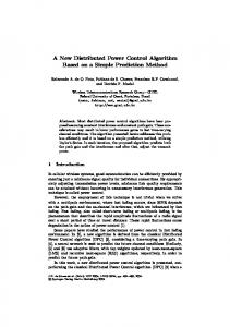
be impossible for many practical systems. More specifically, the optimal power control methods reported in [2] [3] for the case of one secondary source-to-destination (SD) pair sharing the spectrum with one PU were derived by assuming the transmitters to know the instantaneous channel gains of both SU-to-SU and SU-to-PU channels. The results were extended to CR networks with multiple SD pairs [4] and multi-hop relaying SUs [5] based on the similar assumptions. Motivated by these limitations, a game theoretic framework is established in this paper to solve the power control problem of distributed CR networks with multiple secondary SD pairs and PUs. A simple distributed algorithm is proposed to achieve the following advantages: 1) the operations of each SU are simple and fully distributed, i.e., both SUs and PUs do not know the global information, and there is no central controller to manage the network. In addition, each PU in our setting broadcasts the same information to all SUs and each SU cannot communicate with others or obtain specific instructions from PUs, 2) the computational complexity of each SU is low and does not depend on the number of SUs, 3) the proposed algorithm can be directly applied to other resource control problems, e.g., spectrum allocation, time scheduling, etc. It is proved that, the CR network with this simple algorithm can achieve a time average performance as good as that achieved when the Nash equilibrium (NE) is chosen in hindsight. More specifically, we show that by using the proposed algorithm the average performance ( (of))each SU converges to an 𝜖-NE at a rate of 𝑇𝜖 = 𝑂 exp 1𝜖 . This is a surprising result because finding the NE for multi-user networks is generally a challenging task even when the number of users is small [6, Chapter 2], and most of the previously reported NE-approaching algorithms only focus on the instantaneous performance and require more stringent conditions than ours. To further improve the convergence rate, a sub-optimal algorithm is also proposed to (approach a neighborhood of the ) NE at a rate of log𝑇𝜖𝑇′ ′ = 𝑂 𝜖1′ . We discuss some potential 𝜖 extensions of our work and present numerical results to verify the performance of our algorithms for different applications. The rest of this paper is organized as follows. The network model and problem formation are discussed in section II. The proposed algorithm and its convergence result are presented in Sections III. Applications and numerical results are given in Section IV and the paper is concluded in Section V. II. N ETWORK M ODEL AND G AME F ORMULATION Consider a CR network in which 𝐾 secondary SD pairs, labeled as 𝑆1 to 𝐷1 , 𝑆2 to 𝐷2 , ..., 𝑆𝐾 to 𝐷𝐾 , simultaneously transmit signals in the same spectrum as that for 𝑀 PUs, labeled as 𝑃1 , 𝑃2 , ..., 𝑃𝑀 , as shown in Figure

c 2011 IEEE 1536-1276/11$25.00 ⃝

XIAO et al.: A SIMPLE DISTRIBUTED POWER CONTROL ALGORITHM FOR COGNITIVE RADIO NETWORKS

Fig. 1.

Network model for CR networks with multiple SD pairs.

1. Let the channel gain between 𝑆𝑖 and 𝐷𝑗 be ℎ𝑆𝑖 ,𝐷𝑗 for 𝑖, 𝑗 ∈ {1, 2, ..., 𝐾}, and that between 𝑆𝑖 and 𝑃𝑘 be ℎ𝑆𝑖 ,𝑃𝑘 for 𝑖 ∈ {1, 2, ..., 𝐾}, 𝑘 ∈ {1, 2, ..., 𝑀 }. In a practical system, 𝑃𝑘 for 𝑘 ∈ {1, 2, ..., 𝑀 } can only maintain a certain level of QoS if its received interference power is lower than the interference temperature limit, denoted by 𝑞𝑘 . Let the transmit power of 𝑆𝑖 be 𝑤𝑖 . We can define the power constraints for SUs as follows: 𝑯 𝑃 𝑈 𝒘† ≤ 𝒒† , where † denotes the transpose of [𝑤1 , 𝑤2 , . . . , 𝑤𝐾 ], 𝒒 = [𝑞1 , 𝑞2 , . . . , 𝑞𝑀 ], is given by ⎡ ℎ𝑆1 ,𝑃1 ℎ𝑆2 ,𝑃1 ⋅ ⋅ ⋅ ⎢ ℎ𝑆1 ,𝑃2 ℎ𝑆2 ,𝑃2 ⋅ ⋅ ⋅ ⎢ 𝑯𝑃 𝑈 = ⎢ .. .. .. ⎣ . . . ℎ𝑆1 ,𝑃𝑀

ℎ𝑆2 ,𝑃𝑀

(1) a matrix, 𝒘 = and 𝑯 𝑃 𝑈 ∈ ℝ𝑀×𝐾 ℎ𝑆𝐾 ,𝑃1 ℎ𝑆𝐾 ,𝑃2 .. .

⎤ ⎥ ⎥ ⎥. ⎦

(2)

⋅ ⋅ ⋅ ℎ𝑆𝐾 ,𝑃𝑀

Based on the above notations, the received signal to noise ratio (SNR) of 𝐷𝑖 can be written as 𝑆𝑁 𝑅𝑖 =

∑

ℎ𝑆𝑖 ,𝐷𝑖 𝑤𝑖 . ℎ𝑆𝑗 ,𝐷𝑖 𝑤𝑗 + 𝜎𝑖

(3)

𝑗∈{1,2,...,𝐾} 𝑗∕=𝑖

where if PUs keep sending signals during the SUs’ communication, 𝜎𝑖 should contain both the transmit signals of PUs and the additive noise received by 𝑆𝑖 . However, if PUs are absent when SUs transmit, i.e., as in the time sharing spectrum (TSS) based CR networks [7], 𝜎𝑖 should only contain the additive noise of 𝑆𝑖 . In this paper, the game theoretic method is used to investigate the power control problem for CR networks. In our game, players are SUs who share the spectrum with PUs. We define the revenue of the 𝑖th SD pair, denoted by 𝑟𝑖 , to be the benefit obtained by 𝑆𝑖 and 𝐷𝑖 from using the PUs’ spectrum. The price paid by 𝑆𝑖 , denoted by 𝑐𝑖 , is defined as the price charged by PUs for using the licensed spectrum. We also define the payoff of the 𝑖th SD pair, denoted by 𝜋𝑖 , to be the difference between the revenue and price, i.e., 𝜋𝑖 = 𝑟𝑖 − 𝑐𝑖 . In this paper, we assume the revenue and payoff of 𝑆𝑖 to be the function of 𝑆𝑁 𝑅𝑖 defined in (3). Let us consider a finitely repeated game model [8] in which each SU plays the game repeatedly. By using subscript [𝑡] to denote the parameters and operations in the 𝑡th time slot, the main objective of the 𝑖th SD pair is to maximize its

3595

∑ time average payoff 𝑇1 𝑇𝑡=1 𝜋𝑖 (𝒘 [𝑡] ) over 𝑇 time slots of transmission without causing the adverse effects on other SD pairs. This is different from most of the previously reported work in repeated game where each player only cares about the payoff of the last iteration, i.e., payoff in the 𝑇 th time slot. Our setting has more practical meaning for CR networks because most mobile devices can tolerate a few periods of “bad" performance if the average payoff is good. It is assumed that each player cares the performance of the future as same as that of the present and hence the time discount factor [8, Definition 6.1.2] is 1. The result with other choice of the time discount factor can be similarly obtained. The main objective is to find a balance point of the entire network, called Nash Equilibrium (NE), in which each SD pair cannot further improve its payoff by choosing a different transmit power, given the transmit powers of other SUs. The formal definition of the NE is given as follows. Definition 1. [8, Definition 3.3.4] A strategy profile 𝑤𝑖∗ is at a Nash equilibrium (NE) if, for every player 𝑖 and every strategy ∗ ) 𝑤𝑖 , 𝑤𝑖∗ is at least as good as the strategy profile (𝑤𝑖 , 𝑤−𝑖 in which the player 𝑖 chooses 𝑤𝑖 while other players choose ∗ 𝑤−𝑖 , i.e., for every player 𝑖, ∗ ∗ 𝜋𝑖 (𝑤𝑖∗ , 𝑤−𝑖 ) ≥ 𝜋𝑖 (𝑤𝑖 , 𝑤−𝑖 ),

(4)

where subscript −𝑖 means all the players except player 𝑖. We also define a strategy profile to be 𝜖-Nash equilibrium (𝜖-NE), if this strategy profile is within the distance of 𝜖 to the payoff achieved by a NE, i.e., the following condition needs to be satisfied, ( ) ( ) ∗ ∗ − 𝜋𝑖 𝑤𝑖 , 𝑤−𝑖 ≤ 𝜖 for 𝜖 > 0. (5) 𝜋𝑖 𝑤𝑖∗ , 𝑤−𝑖 Finding the NE of the multi-user network is difficult and intractable [6, Chapter 2]. In this paper, we try to develop an algorithm that, during 𝑇 time slots of repeated power control games, can achieve the average performance nearly as good as the system with the NE decision being chosen in hindsight, i.e., we have 𝑇 2 ( ) 1 ∑ min 𝝅 𝒘[𝑙] − 𝝅 (𝒘∗ ) 2 = 0 𝑇 →∞ 𝑇 𝑙∈{1,...,𝑡} 𝑡=1 [ ] where 𝝅(𝒘 [𝑙] ) = 𝜋1 (𝒘[𝑙] ), 𝜋2 (𝒘 [𝑙] ), ..., 𝜋𝐾 (𝒘[𝑙] ) .

lim

(6)

III. M AIN R ESULTS Algorithm 1 is illustrated below. 1) Initialization: Let the transmit signal of 𝑆𝑖 be 𝑥𝑖 . Consider the transmission of the 𝑖th SD pair. During the first two time slots, i.e., 𝑡 ∈ {1, 2}, a) 𝑆𝑖 first sends signals 𝑥𝑖[1] and 𝑥𝑖[2] with powers 𝑤𝑖[1] and 𝑤𝑖[2] , respectively, b) After receiving the signal sent by 𝑆𝑖 , 𝐷𝑖 , observed its received SNR, feedbacks the revenue functions 𝑟𝑖[1] and 𝑟𝑖[2] in the first and second time slots, respectively. Each PU 𝑃𝑘 also sends the prices 𝑐𝑘[1] and 𝑐𝑘[2] to 𝑆𝑖 during the first two time slots. 2) Iteration: For 𝑡 = 3 : 𝑇 , a) In ∑𝐾time slot 𝑡, 𝑃𝑘 monitors its interference power 𝑖=1 ℎ𝑆𝑖 ,𝑃𝑘 𝑤𝑖[𝑡] . If the interference powers of all

3596

IEEE TRANSACTIONS ON WIRELESS COMMUNICATIONS, VOL. 10, NO. 11, NOVEMBER 2011

PUs satisfy (1), 𝑃𝑘 only sends price 𝑐𝑖[𝑡] to 𝑆𝑖 , and then 𝑆𝑖 updates its transmit power as follows, )+ ( (7) 𝑤𝑖[𝑡] = 𝑤𝑖[𝑡−1] − 𝛿𝑖[𝑡−1] 𝑔𝑖[𝑡] , where (⋅)+ = max{0, ⋅}, 𝑔𝑖[𝑡] is a subgradient [9] of 𝜋𝑖[𝑡] which is a function that satisfies the relation ( ) ( ) ≥ 𝜋𝑖[𝑡−1] 𝒘[𝑡−1] 𝜋𝑖[𝑡] 𝒘[𝑡] ( ) +𝑔𝑖[𝑡] 𝒘[𝑡] − 𝒘 𝑖[𝑡−1] , (8) and 𝛿𝑖[𝑡−1] is the step size of the 𝑡th iteration, defined 𝑢𝑖 as 𝛿𝑖[𝑡−1] = 𝑡−1 where 𝑢𝑖 is the step size coefficient which is a constant controlling the iteration speed, b) However, if the interference powers of some PUs exceed the interference temperature limit, each of these PUs should transmit more information to help SUs to adjust the transmit powers during the subsequent iterations. More specifically, ∑ assuming 𝑃𝑘 observes 𝐾 high interference power, i.e., 𝑖=1 ℎ𝑆𝑖 ,𝑃𝑘 𝑤𝑖[𝑡] > 𝑞𝑘 , the operations of 𝑃𝑘 , except for sending the price to SUs, are described as follows, i) 𝑃𝑘 broadcasts a high-interference-message to inform all SUs that its interference power exceeds the limit. 𝑆𝑖 can decode this message and exploit it to obtain ℎ𝑆𝑖 ,𝑃𝑘 , ii) Because we assume each PU monitors its interference power in each iteration, 𝑃𝑘 can calculate the interference power exceeding value 𝐼𝑘[𝑡] =

𝐾 ∑

ℎ𝑆𝑖 ,𝑃𝑘 𝑤𝑖[𝑡] − 𝑞𝑘 ,

(9)

𝑖=1

and the change of interference power in time slot 𝑡 𝐽𝑘[𝑡] =

𝐾 ∑

ℎ𝑆𝑖 ,𝑃𝑘 𝑤𝑖[𝑡] −

𝑖=1

𝐾 ∑

ℎ𝑆𝑖 ,𝑃𝑘 𝑤𝑖[𝑡−1] , (10)

𝑖=1

iii) By assuming the channel gains to be known by the receivers (i.e., assume a training code is involved in the transmit signals of SUs), 𝑃𝑘 can exploit its received signal to calculate a constant ∑𝐾 Φ𝑘[𝑡] = 𝑖=1 ℎ2𝑆𝑖 ,𝑃𝑘 . Each PU 𝑃𝑘 broadcasts the constants 𝐼𝑘[𝑡] , 𝐽𝑘[𝑡] and Φ𝑘[𝑡] to all SUs, iv) 𝑆𝑖 , knowing ℎ𝑆𝑖 ,𝑃𝑘 (obtained in Step b-i)), updates its transmit power by 𝑤𝑖[𝑡]

=

[

𝑤𝑖[𝑡−1] − 𝛿𝑖[𝑡−1] 𝑔𝑖[𝑡] (11) ( )]+ −1 −ℎ𝑆𝑖 ,𝑃𝑘 Φ𝑘[𝑡−1] 𝐼𝑘[𝑡−1] − 𝐽𝑘[𝑡−1] .

If more than one PU detects higher-than-tolerate interference power, they should sequentially repeat the operations from Steps b-i) to b-iv) until the transmit powers of all SUs satisfy (1). 3) Termination: The above process continues until the obtained payoff is close to the optimal value within an acceptable range, i.e., ∥𝜋𝑖[𝑡] (𝒘 [𝑡] ) − 𝜋𝑖[𝑡] (𝒘∗ )∥22 ≤ 𝜖, or the number of time slots reaches 𝑇 , i.e., 𝑡 = 𝑇 . The main idea of Algorithm 1 is that if the transmit powers of SUs satisfy (1), each SU maximizes its payoff by using

the subgradient method, as shown in Step 2-a). If any PUs detect the higher-than-tolerable interference levels, they will broadcast several constants, i.e., 𝑃𝑘 broadcasts Φ𝑘 , 𝐼𝑘 and 𝐽𝑘 defined in Step 2) to all SUs, and SUs use these constants to project their transmit powers into the convex hull defined in (1). Note that simply projecting the transmit powers of all SUs to (1) requires each PU to know the information of all other PUs, which does not meet the requirements that PUs cannot communicate with each other. Hence, in Algorithm 1, if more than one PU detect higher-than-tolerable interference power, each of them informs SUs to project their powers to the corresponding linear equation in the convex hull defined in (1) one by one. This setting will not result in much adverse effects on the convergence performance of Algorithm 1 because we always assume 𝑇 ≫ 𝐾. Also if the transmit powers of SUs increase gradually, only a few PUs will first detect high-thantolerable interference powers in each time slot. In other words, the number of iterations used on the projection operation is negligible as the total number of iterations becomes large. Note that our algorithm is different from that proposed in [10] in which each SU needs to communicate with its nearby SUs to make decisions based on the “consensus" among them. In our algorithm, each PU (or SU) cannot communicate with its nearby PUs (or SUs), and hence can be directly applied into many practical systems, i.e., the cellular based mobile network. Theorem 1. If the following assumptions A1) The iteration step sizes are bounded, i.e., ∥𝑔𝑖[𝑡] ∥22 ≤ 𝑔𝑖+ , where 𝑔𝑖+ is a constant, A2) The difference of power values between two iterations is bounded, i.e., ∥𝑤𝑖[𝑡] − 𝑤𝑖[𝑠] ∥22 ≤ 𝑤𝑖+ for 𝑡 ∕= 𝑠 and 𝑡, 𝑠 ∈ {1, ..., 𝑇 }, where 𝑤𝑖+ is a constant, A3) The payoff for the 𝑖th SD pair is a continuous function of 𝑤𝑖 , are satisfied, then Algorithm 1 has the following properties P1) It converges to a stationary point if 𝑇 is large enough, P2) If all SD pairs use Algorithm 1, the time average payoff of 𝑆𝑖 converges to an 𝜖-NE at a rate of ( ( )) 𝑂 exp 1𝜖 1 , i.e., 2 𝑇𝜖 1 ∑ ) ( 𝝅 𝒘[𝑡] − 𝝅 (𝒘∗ ) ≤ 𝜖. (12) 𝑇𝜖 𝑡=1

2

Proof: See Appendix A. Note that the convergence performance of Algorithm 1 is closely related to the combination of two important parameters: the initial value 𝑤𝑖[1] of transmit powers and the iteration step size 𝑢𝑖 . If 𝑤𝑖[1] and 𝑢𝑖 satisfies ∣𝑤𝑖[1] − 𝑤𝑖∗ ∣ ≈ 𝑢𝑖 , Algorithm 1 could approach to the neighborhood of a NE within a few iterations. However, if 𝑤𝑖[1] and 𝑢𝑖 are improperly chosen, the convergence rate of Algorithm 1 will be very slow. This slow convergence rate is due to the fact that we require 𝑤𝑖 to reach 𝑤𝑖∗ exactly without assuming any information about the systems or channel gains to be known by SUs. The slow 1 In this paper, we follows Bachmann-Landau notations: 𝑓 = 𝑂(𝑔) if (𝑛) < +∞. lim 𝑓𝑔(𝑛)

𝑛→∞

XIAO et al.: A SIMPLE DISTRIBUTED POWER CONTROL ALGORITHM FOR COGNITIVE RADIO NETWORKS

𝑤𝑖+ 𝐿

and 𝑤𝑖[𝑡] is calculated by using either (7) (if the power constraint in (1) is satisfied) or (11) (if (1) is not satisfied) in Algorithm 1. The NE is a balance point where each player achieves locally optimal solution and hence has no incentive to deviate from this point. In other words, we can always find a neighborhood, denoted as 𝝌 = [𝜒1 , 𝜒2 , ..., 𝜒𝐾 ], for the NE that all the elements in this neighborhood cannot achieve ∗ )≥ higher performance than that of the NE, i.e., 𝜋𝑖 (𝑤𝑖∗ , 𝑤−𝑖 ∗ 𝜋𝑖 (𝒘 ± Δ𝒘) where Δ𝒘 = [Δ𝑤1 , Δ𝑤2 , ..., Δ𝑤𝐾 , ] and 0 < Δ𝑤𝑖 < 𝜒𝑖 for 𝑖 ∈ {1, 2, ..., 𝐾}. It is easy to observe that if 𝒘 [𝑡] − 𝒘[𝑡+1] > 𝝌, Algorithm 2 may not converge to a NE. Let us summarize our observations and present the main result for Algorithm 2 as follows. 𝛿ˆ 𝑔+

Theorem 2. If 𝑤𝑖 ∈ 𝒲𝑖 , 𝜒𝑖 ≫ 𝑖2 𝑖 ∀ 𝑖 ∈ {1, 2, ..., 𝐾} and Assumptions A1)-A3) 1 ]are satisfied, Algorithm 2 [ ˆ + ˆin +Theorem + 𝛿ˆ𝐾 𝑔𝐾 𝛿1 𝑔1 𝛿2 𝑔2 neighborhood of a NE, approaches a 2 , 2 , ..., 2 ) ( ) 2 ( 𝜖′ 1 𝑇∑ 𝛿ˆ𝑖 𝑔𝑖+ 𝛿ˆ𝑖 𝑔𝑖+ ∗ ∗ −𝝅 𝒘 ± 2 ≤ i.e., 𝑇 ′ 𝝅 𝑤𝑖[𝑡] , 𝑤−𝑖[𝑡] ± 2 𝜖 𝑡=1 2 (1) 𝛿ˆ𝑖 𝑔𝑖+ 𝑇𝜖′ ′ ′ 𝜖 , at a rate of log 𝑇 ′ = 𝑂 𝜖′ , where 𝜖 = ∣𝜖 − 2 ∣ and 𝜖 𝑤+ 𝛿ˆ𝑖 = 𝑖 . 𝐿

Proof: See Appendix B. IV. A PPLICATIONS AND N UMERICAL R ESULTS In this section, the proposed algorithm is applied to the network utility maximization problem to evaluate its performance. We assume that each SU has an objective to maximize its achievable rate and define the utility function of 𝑆𝑖 as 𝑟𝑖 (𝑤𝑖 ) = 𝛾𝑖 log (1 + 𝑆𝑁 𝑅𝑖 ) where 𝑆𝑁 𝑅𝑖 is defined in (3) and 𝛾𝑖 is a constant. Since Algorithm 2 can be regarded as a special case of Algorithm 1, we only present the numerical results for Algorithm 1. Consider a special case where SUs are far from each other ℎ 𝑤 𝑖 𝑖 . Assume PUs do not charge any and 𝑆𝑁 𝑅𝑖 ≈ 𝑆𝑖 ,𝐷 𝜎𝑖 prices for SUs if the transmit powers of SUs satisfy (1). It

0.6

t=1

Average Revenue: (1/T) Σ T r[t]

convergence performance of Algorithm 1 can be improved by assuming more information to be observed by SUs. For example, if we assume that 𝑆𝑖 knows the payoff functions, or both the revenue and pricing functions, the optimization problem can be converted into the Lagrangian dual problem [11] which will be discussed in the next section. Another way to improve the convergence rate of Algorithm 1 is to decrease the required accuracy of the results. In practical digital systems, mobile devices cannot adjust their parameters with an infinite accuracy, i.e., the value of 𝑤𝑖 can only be chosen from a finite discrete set. In the rest of this section, we consider a simple case in which the transmit power of each SU is linearly quantized into 𝐿 levels and 𝑤𝑖 can only be chosen from this finite set, i.e., 𝑤𝑖 ∈ 𝒲𝑖 where 𝑤 + 2𝑤 + 𝒲𝑖 = {0, 𝐿𝑖 , 𝐿𝑖 , ..., 𝑤𝑖+ }. Let us describe Algorithm 2 as follows. Algorithm 2: Each SU adjusts its transmit power by using the exact same procedures as Algorithm 1. The only difference is that, in the 𝑡th iteration, the transmit power of 𝑆𝑖 is 𝑤𝑖[𝑡] = ˆ ˆ 𝑙𝛿ˆ𝑖 if 𝑙𝛿ˆ𝑖 − 𝛿2𝑖 < 𝑤𝑖[𝑡] < 𝑙𝛿ˆ𝑖 + 𝛿2𝑖 where 𝑙 ∈ {1, 2, ..., 𝐿}, 𝛿ˆ𝑖 =

3597

0.5

0.4 u=2 u=4 u=6 Dual Method Optimal Value

0.3

0.2

0.1

0

0

20

40

60

80 Iteration

100

120

140

Fig. 2. Comparison of different algorithms, where 𝑀 = 1, 𝐾 = 10, 𝑞𝑘 = 2, for 𝑖 ∈ {1, 2, ..., 𝐾}, 𝑘 ∈ {1, 2, ..., 𝑀 }.

is observed that in this case the payoff function 𝜋𝑖 (𝒘) of 𝑆𝑖 has the following features: 1) it is continuous in 𝒘, 2) it is concave in 𝑤𝑖 , 3) it has a continuous first derivative with respect to 𝑤𝑖 , and 4) there exists 𝑟 = {𝑟1 , 𝑟2 , ..., 𝑟𝐾 } > 0 such ∑𝐾 that 𝑖=1 𝑟𝑖 𝜋𝑖 (𝒘) is diagonally strictly concave. Following the same methods as in [12], we can claim that for this CR network the NE is unique and corresponds to the global utility maximization point [11]. In other words, if all SUs use Algorithm 1 to adjust their transmit powers, the average payoff of the network will converge to the global utility maximization 𝑇 ( ) ∑ ∑𝐾 1 𝜋[𝑡] 𝒘 [𝑡] for 𝜋[𝑡] = 𝐾 point, defined as max 𝑇1 𝑖=1 𝜋𝑖[𝑡] 𝒘

𝑡=1

under the power constraint defined in (1). To demonstrate the convergence performance of Algorithm 1, the results of the Lagrangian dual methods discussed in [11] are also provided. In this method, 𝑆𝑖 iteratively chooses the optimal Lagrangian coefficients to maximize its payoff (see [11] for the detailed description of the dual method). In Figure 2, we compare the convergence rates of Algorithm 1 and the dual method. It is observed that the dual method generally converges to the optimal value at a faster rate than Algorithm 1. However, each SU in the dual method needs to know the payoff functions of all SUs and has to search for the optimal power to minimize the objective function in each iteration, which incurs much more computational complexity and communication overhead than those of our proposed algorithm. In addition, Figure 2 shows that if the step size is chosen optimally, the convergence rate of Algorithm 1 could outperform that of the dual methods. Let us consider a more general case as follows. Define the revenue of 𝑆𝑖 as 𝑟𝑖 = 𝛼𝑖 log (1 + 𝑆𝑁 𝑅𝑖 ) where 𝑆𝑁 𝑅𝑖 is given in (3) and 𝛼𝑖 is a constant. The pricing function charged 𝑀 ∑ by all PUs from 𝑆𝑖 is given by 𝑐𝑖 = 𝛽𝑖 ℎ𝑆𝑖 ,𝑃𝑘 𝑤𝑖 where 𝑘=1

𝛽𝑖 is a constant. Note that this problem is not convex and is generally impossible to efficiently find the global optimal solution [13]. In this case, Algorithm 1 may not converge to the global utility maximization point, but still can converge to a NE. The convergence results of Algorithm 1 with different parameters in this case are presented in Figures 3 and 4. As

3598

IEEE TRANSACTIONS ON WIRELESS COMMUNICATIONS, VOL. 10, NO. 11, NOVEMBER 2011

0.14

1

0.12

0.9

w decided by the PUs (w = h

0.1

Average Payoff: (1/T) ΣT π[t]

u=1.5 u=2 u=2.5 u=3

0.08 0.06

i[1] S ,P i

\q )

k

k

0.8

t=1

Average Payoff: (1/T) ΣT π

t=1 [t]

i[1]

Power Control with Algorithm 1 (400 iterations) Power Control with Algorithm 1 (300 iterations) Power Control with Algorithm 1 (200 iterations) Power Control with Algorithm 1 (100 iterations)

0.04 0.02 0

0.7 0.6 0.5 0.4 0.3

−0.02 −0.04

50

100 150 Number of Iterations

200

250

0.2

1

1.5

2

2.5

3 3.5 Distance dS ,D i

Fig. 3. Convergence rate of Algorithm 1 with different step sizes, where 𝑤𝑖[1] is the least squares solution of 𝑯 𝑃 𝑈 𝒘 † = 𝒒 † , 𝛼𝑖 = 10, 𝛽𝑖 = 0.1, 𝑀 = 5, 𝐾 = 10, 𝑞𝑘 = 5, for 𝑖 ∈ {1, 2, ..., 𝐾}, 𝑘 ∈ {1, 2, ..., 𝑀 }.

4

4.5

5

i

Fig. 5. Payoffs of power control achieved by Algorithm 1 and fixed transmit power (𝑤𝑖[1] = ℎ𝑆𝑖 ,𝑃𝑘 ∖𝑞𝑘 ) under different 𝑑𝑆𝑖 ,𝐷𝑖 , where 𝛼𝑖 = 10, 𝛽𝑖 = 0.1, 𝑀 = 5, 𝐾 = 10, 𝑞𝑘 = 2, 𝑢𝑖 = ∥𝑔 1 ∥2 , for 𝑖 ∈ {1, 2, ..., 𝐾}, 𝑘 ∈ {1, 2, ..., 𝑀 }.

𝑖[𝑡] 2

−0.14 −0.16

Average Payoff: (1/T) ΣT π

t=1 [t]

−0.18

wi[1] = 0.75*hik\q

−0.2

wi[1] = hik\q wi[1] = 1.5* hik\q

−0.22

wi[1] = 2* hik\q

−0.24 −0.26 −0.28 −0.3 −0.32 −0.34

0

100

200 300 Number of Iterations

400

500

Fig. 4. Convergence rate of Algorithm 1 with different initial values, where 𝑤𝑖[1] = ℎ𝑆𝑖 ,𝑃𝑘 ∖𝑞𝑘 means 𝑤𝑖[1] is the least squares solution of 𝑯 𝑃 𝑈 𝒘† = 𝒒, 𝛼𝑖 = 10, 𝛽𝑖 = 0.1, 𝑀 = 5, 𝐾 = 10, 𝑞𝑘 = 5, 𝑢𝑖 = ∥𝑔 1 ∥2 , for 𝑖 ∈ {1, 2, ..., 𝐾}, 𝑘 ∈ {1, 2, ..., 𝑀 }.

𝑖[𝑡] 2

observed in Section III, the convergence rate of Algorithm 1 depends on the initial transmit powers of SUs and the iteration step size. It is observed that if 𝑤𝑡[1] has a distance of 𝑢𝑖 from a NE, only a few number of iterations are required to approach the performance of this NE. However, if the initial transmit powers are not properly chosen, the adjustment of Algorithm 1 on the transmit powers of SUs may require a large number of iterations. Similarly, an optimal value of 𝑢𝑖 should be close to the distance between 𝑤𝑖[1] and 𝑤𝑖∗ . However, if no information about initial transmit power and the optimal power are known, on one hand, a large step size may lead to high fluctuations during the first few iterations and, on the other hand, a small step size will cause slow convergence rate. The above observation shows the importance of choosing proper combinations of initial powers and step sizes. In a practical system, SUs can first send the training code to let PUs to decide proper initial values of SUs’ transmit powers. Also, the step size of each iteration, chosen by each SD pair, can

be adjusted if more information can be observed or more feedback messages can be received during the communication, i.e., the dual methods. Finding the distributed algorithms to allow iterative improvement of the step size in Algorithm 1 will be our future work. Let us consider the numerical results of CR networks with Algorithm 1. Denote the distance between two users 𝑝 and 𝑞 as 𝑑𝑝,𝑞 for 𝑝, 𝑞 ∈ [𝑆1 , 𝑆2 , ..., 𝑆𝐾 ] ∪ [𝐷1 , 𝐷2 , ..., 𝐷𝐾 ] ∪ [𝑃1 , 𝑃2 , ..., 𝑃𝑀 ] and consider the following channel models, 𝜂 ˜ 𝑖𝑗 /𝑑𝜂 ˜ ˜ ℎ𝑖𝑗 = ℎ 𝑆𝑖 ,𝐷𝑗 and ℎ𝑖𝑘 = ℎ𝑖𝑘 /𝑑𝑆𝑖 ,𝑃𝑘 , where ℎ𝑖𝑗 and ˜ ℎ𝑖𝑘 are average channel fading coefficients unrelated to the distance of the transmission and 𝜂 is the channel attenuation exponent. Assume that SUs are located on a regular planar network, i.e., 𝑑𝑆𝑖 ,𝑃𝑘 = 𝑑𝑆𝑗 ,𝑃𝑙 , 𝑑𝑆𝑖 ,𝐷𝑖 = 𝑑𝑆𝑗 ,𝐷𝑗 , √ 2 𝑑𝑆𝑖 ,𝑆𝑗 + 𝑑2𝑆𝑗 ,𝐷𝑗 and 𝑑𝑆𝑖 ,𝑆𝑖+1 = 𝑑𝐷𝑗 ,𝐷𝑗+1 , for 𝑑𝑆𝑖 ,𝐷𝑗 = 𝑖, 𝑗 ∈ {1, 2, ..., 𝐾} and 𝑘, 𝑙 ∈ {1, 2, ..., 𝑀 }. In Figure 5, the average payoff of the network obtained by using Algorithm 1 with different 𝑑𝑆𝑖 ,𝐷𝑖 is shown and compared with that of the fixed transmit power method. It is observed that the proposed algorithm greatly improves the performance of CR networks. More importantly, even with a small number of iterations, Algorithm 1 can achieve a significant payoff improvement.

V. C ONCLUSION In this paper, the power control problem for SSS based CR networks with multiple secondary SD pairs and PUs has been investigated. A simple distributed algorithm has been proposed to iteratively improve the performance of CR networks. It has been proved that the proposed converges to an 𝜖)) ( ( algorithm NE at a speed of 𝑇𝜖 = 𝑂 exp 1𝜖 . A sub-optimal algorithm has been also proposed to converge ( ) to a neighborhood of a NE at a rate of log𝑇𝜖𝑇′ ′ = 𝑂 𝜖1′ . Numerical results have 𝜖 been presented to show the convergence rates under different settings.

XIAO et al.: A SIMPLE DISTRIBUTED POWER CONTROL ALGORITHM FOR COGNITIVE RADIO NETWORKS

{ 𝒘[𝑡+1] =

𝒘[𝑡] − 𝛿[𝑡] 𝒈 [𝑡] ,

( )−1 ( ) 𝑯 𝑃 𝑄 𝒘[𝑡] − 𝑯 𝑃 𝑄 𝜹 [𝑡] 𝒈 [𝑡] − 𝒒 , 𝒘[𝑡] − 𝛿[𝑡] 𝒈 [𝑡] − 𝑯 †𝑃 𝑄 𝑯 𝑃 𝑄 𝑯 †𝑃 𝑄

A PPENDIX A P ROOF OF T HEOREM 1

1 𝑇

𝑡=1

=

(𝑏)

≤

(𝑎)

∥𝒘[𝑡+1] − 𝒘∗ ∥22 =

1 𝑇

𝑇 ∑

∥𝒘[𝑡] − 𝒘 ∗ − 𝜹 [𝑡] 𝒈 [𝑡] ∥22

𝑡=1

𝑇 ( ) 1 ∑[ ∥𝒘[𝑡] − 𝒘∗ ∥22 − 2𝜹 [𝑡] 𝒈 [𝑡] 𝒘[𝑡] − 𝒘 ∗ 𝑇 𝑡=1 ] +𝜹 2[𝑡] ∥𝒈 [𝑡] ∥22 𝑇 ) ( ( ) 1 ∑[ ∥𝒘[𝑡] − 𝒘 ∗ ∥22 − 2𝜹 [𝑡] 𝝅 𝒘 [𝑡] − 𝝅 (𝒘∗ ) 𝑇 𝑡=1 ] +𝜹 2[𝑡] ∥𝒈 [𝑡] ∥22 , (14)

where (𝑎) and (𝑏) are obtained by using (7) and (8) in Algorithm 1, respectively. Equation (14) can be rewritten recursively as follows: 𝑇 1 ∑ 𝒘 [𝑡+1] − 𝒘∗ 2 ≤ 𝒘[1] − 𝒘 ∗ 2 2 2 𝑇 𝑡=1

−

𝑇 𝑡 ( ( ) ) 2 ∑∑ 𝜹 [𝑙] 𝝅 𝒘[𝑙] − 𝝅 (𝒘 ∗ ) 𝑇 𝑡=1 𝑙=1

𝑇 𝑡 1 ∑∑ 2 2 + 𝜹 [𝑙] 𝒈 [𝑙] . 𝑇 𝑡=1 2

if 𝑯 𝑃 𝑈 𝒘[𝑡] ≤ 𝒒 𝑗 ,

(13)

otherwise,

as follows:

From Definition 1, it is observed that for a NE, a neighborhood can always be found in which all the elements in this neighborhood have lower payoff than the NE. By assuming all payoff functions of SUs to be continuous, the neighborhood of the NE can be regarded as a quasiconcave hull, i.e., for 𝝌 = [𝜒1 , 𝜒2 , ..., 𝜒𝐾 ] neighborhood of a NE, we have 𝜋𝑖 (𝒘∗ ± Δ𝒘) < 𝜋𝑖 (𝒘) where 𝒘 ∈ [𝒘∗ − Δ𝒘, 𝒘∗ + Δ𝒘] and Δ𝑤𝑖 ≤ 𝜒𝑖 . Since Algorithm 1 uses a decreasing step size for iteration, it will finally fall into a small neighborhood of the NE. Therefore, if Algorithm 1 is proved to converge to a stationary point in which all elements in a neighborhood of that point has lower payoffs, we can claim that this point is the NE and Algorithm 1 converges. Defining 𝒈 [𝑡] = [𝑔1[𝑡] , 𝑔2[𝑡] , ..., 𝑔𝐾[𝑡] ]† , we can re-write (11) in Algorithm 1 to the vector form in (13) at the top of next page. In this figure, 𝑯 𝑃 𝑄 is a sub-matrix of 𝑯 𝑃 𝑈 which only contains the channel gains connected with one PU observing high interference noises in its rows, and 𝜹 [𝑡] = diag[𝛿1[𝑡] , 𝛿2[𝑡] , ..., 𝛿𝐾[𝑡] ]. Let us first consider the case that the transmit powers of the SUs always satisfy (1). Denoting a NE achieving power ∗ † ] , control schemes for all the SUs as 𝒘 ∗ = [𝑤1∗ , 𝑤2∗ , ..., 𝑤𝐾 we have 𝑇 ∑

3599

(15)

𝑙=1

∑𝑇 Note that we have 𝑇1 𝑡=1 ∥𝒘[𝑡+1] − 𝒘∗ ∥22 ≥ 0, and the second term in the right-hand-side of (15) can be expressed

𝑇 𝑡 ( ( ) ) 2 ∑∑ 𝜹 [𝑙] 𝝅 𝒘[𝑙] − 𝝅 (𝒘∗ ) (16) 𝑇 𝑡=1 𝑙=1 ( 𝑡 ) 𝑇 ] [ ( ) 2 ∑ ∑ ≥ 𝜹 [𝑙] min 𝝅 𝒘[𝑙] − 𝝅 (𝒘∗ ) 𝑇 𝑡=1 𝑙∈[1,𝑡] 𝑙=1 ( ) 𝑇 𝑇 𝑡 (𝑐) [ ( ) ] 2 ∑∑ 1∑ ≥ 𝜹 [𝑙] min 𝝅 𝒘[𝑙] − 𝝅 (𝒘 ∗ ) 𝑇 𝑡=1 𝑇 𝑡=1 𝑙∈[1,𝑡] 𝑙=1

where (𝑐) comes from that fact that ∑𝑇 ∑𝑡 1 1 𝑡=1 𝑙=1 𝑙 . 𝑇 Substituting (16) into (15), we have 𝑇 [ ( ) ] 1 ∑ min 𝝅 𝒘 [𝑡] − 𝝅 (𝒘∗ ) 𝑇 𝑡=1 𝑙∈[1,𝑡]

≤

𝒘[1] − 𝒘 ∗ 2 + 2 2 𝑇

1 𝑇

𝑇 ∑

𝑇 ∑ 𝑡 ∑

𝑡=1 𝑙=1 𝑡 ∑

𝑡=1 𝑙=1

∑𝑡

1 𝑙=1 𝑙

2 𝜹 2[𝑙] 𝒈 [𝑙] 2

.

≥

(17)

𝜹 [𝑙]

Substituting the step size function 𝜹 [𝑙] = 𝒖𝑙 for 𝒖 = [𝑢 equation and using the result ∑] ∞into1 the above ∑1𝑡, 𝑢2 ,1..., 𝑢𝐾 𝜋 < = , and the properties of Harmonic 𝑙=1 𝑙2 ∑ 𝑙=1 𝑙2 6 𝑡 1 −1 1 −2 1 number: − 12 𝑡 + 𝑂(𝑡−4 ) ≈ 𝑙=1 𝑙 = log 𝑡 + 2 𝑡 1 −1 1 −2 ˙ the following results can be obtained: log 𝑡+ 2 𝑡 − 12 𝑡 + 𝜅, 𝑇 ] [ ( ) 1 ∑ min 𝝅 𝒘[𝑙] − 𝝅 (𝒘∗ ) 𝑇 𝑡=1 𝑙∈[1,𝑡] + ∑𝑇 𝜋 (𝑑) 𝒘 + + 𝒘𝑇 𝑡=1 6 ≤ 2 ∑𝑇 −1 + 𝜅) ˙ 𝑡=1 (log 𝑡 + 0.5𝑡 𝑇 𝜅 ¨ ≈ 2 ∑𝑇 log 𝑇 +0.5𝑇 −1 +𝜅˙ log 𝑡 + + 2𝜅˙ 𝑡=1 𝑇 𝑇

(18)

where (𝑑) is obtained from Assumptions A1) and A2) in Theorem 1, and ∑ 𝜅 ¨ is a constant defined as 𝜅 ¨ = 𝒘+ + 𝑇 +𝜋 2 and hence 𝒈 6 . Because 𝑡=1 log 𝑡 = Θ(𝑇 log 𝑇 ) ∑𝑇 log 𝑇 +0.5𝑇 −1 1 → lim𝑇 →∞ 𝑇 𝑡=1 log 𝑡 → ∞ and lim𝑇 →∞ 𝑇 0, it can be claimed that Algorithm 1 converges to a stationary point. Assume that for 𝑇 ≥ 𝑇𝜖 and 𝑇𝜖 is a very large number, we try to achieve the accuracy of 𝑇 [ ( ) ] ∑ 1 min 𝝅 𝒘[𝑙] − 𝝅 (𝒘∗ ) = 𝜖. From (18) and con𝑇 𝑡=1 𝑙∈[1,𝑡]

cavity of logarithm function, the following results can be 2 Again, we follow Bachmann-Landau notations: 𝑓 = Θ(𝑔) if 𝑓 = 𝑂(𝑔) and 𝑔 = 𝑂(𝑔)

3600

IEEE TRANSACTIONS ON WIRELESS COMMUNICATIONS, VOL. 10, NO. 11, NOVEMBER 2011

obtained, 𝜅 ¨ 𝜖

𝑇𝜖 log 𝑇𝜖 + 0.5𝑇𝜖−1 1 ∑ log 𝑡 + + 2𝜅˙ ≥ lim 𝑇𝜖 →∞ 𝑇𝜖 𝑇𝜖 𝑡=1 ( ) ( ) 𝑇𝜖 𝑇𝜖 + 1 1 ∑ = lim log 𝑡 = log 𝑇 →∞ 𝑇𝜖 𝑡=1 2 ( ( )) 1 ⇒ 𝑇𝜖 = 𝑂 exp . 𝜖

Therefore, we can claim that by using Algorithm 1, the average payoff )) networks converges to 𝜖-NE at a speed ( of ( SU of 𝑇𝜖 = 𝑂 exp 1𝜖 . Consider the case that at least one PU observes the higherthan-tolerable interference power. By multiplying (13) with 𝑯 𝑃 𝑄 , it can be easily shown that 𝑯 𝑃 𝑄 𝒘†[𝑡+1] always converges to 𝒒 † . Substituting 𝑯 𝑃 𝑄 𝒘†[𝑡+1] = 𝒒 † into (13), (13) ˜ [𝑡+1] 𝒈 [𝑡+1] , can be rewritten as 𝒘[𝑡+2] = 𝒘 [𝑡+1] − 𝜹 [𝑡+1] 𝒈 ( )−1 ˜ [𝑡+1] = 𝑰 + 𝑯 †𝑃 𝑄 𝑯 𝑃 𝑄 𝑯 †𝑃 𝑄 𝑯 𝑃 𝑄 and 𝑰 is where 𝒈 the identity matrix. If we denote 𝒈 [𝑡] = 𝒈˜ [𝑡] 𝒈 [𝑡] and assume ∥˜ 𝒈 [𝑡] 𝒈 [𝑡] ∥22 ≤ 𝒈 + , the same method as the previous case can be used to obtain the similar convergence rate.

A PPENDIX B P ROOF OF T HEOREM 2 Following the same steps as in Appendix A, let us consider the case in which each SU can only choose from 𝐿 quantized power levels, i.e., 𝑤𝑖 ∈ 𝒲𝑖 . In this case, if the initial point is not appropriately chosen, Algorithm 2 will be unstable for the first few iterations, i.e., fluctuating between different neighborhood of NEs. However, when the number of iterations is large, the transmit powers of SUs will approach to the neighborhood of a NE. Therefore, for a large number of iterations, Algorithm 2 can be regarded as Algorithm 1 with + a constant step size 𝜹 [𝑙] = 𝜹ˆ where 𝜹ˆ = 𝒘𝐿 is a constant. Let us substitute this step size in (17), the following results can be obtained,

𝑇 [ ( ) ] 1 ∑ min 𝜋 𝒘[𝑙] − 𝜋 (𝒘∗ ) 𝑇 𝑡=1 𝑙∈[1,𝑡]

≤

∑𝑡 2 𝑇 1 ∑ 𝒘+ + (𝜹ˆ 𝒈 + /𝑡) 𝑙=1 𝑙 ˆ ∑𝑡 𝑙 𝑇 𝑡=1 (2𝜹/𝑡) 𝑙=1

2 𝑇 1 ∑ 𝒘+ + 𝜹ˆ 𝒈 + (𝑡 + 1) = . 𝑇 𝑡=1 2𝜹ˆ (𝑡 + 1)

(19)

By using the same method as in Appendix A, we can claim that if the step size is fixed, the number of iterations for ( ) ˆ + 𝑇′ Algorithm 2 is given by log𝜖𝑇 ′ = 𝑂 𝜖1′ where 𝜖′ = 𝜖 − 𝜹𝒈2 𝜖 + and 𝜹ˆ = 𝒘 . 𝐿

R EFERENCES [1] S. Haykin, “Cognitive radio: brain-empowered wireless communications,” IEEE J. Sel. Areas Commun., vol. 23, pp. 201–220, 2005. [2] G. Amir and S. S. Elvino, “Fundamental limits of spectrum-sharing in fading environments,” IEEE Trans. Wireless Commun., vol. 6, no. 2, pp. 649–658, 2007. [3] M. Gastpar, “On capacity under receive and spatial spectrum-sharing constraints,” IEEE Trans. Inf. Theory, vol. 53, no. 2, pp. 471–487, 2007. [4] Z. Lan, Y.-C. Liang, and X. Yan, “Joint beamforming and power allocation for multiple access channels in cognitive radio networks,” IEEE J. Sel. Areas Commun., vol. 26, pp. 38–51, 2008. [5] Y. Xiao, G. Bi, and D. Niyato, “Game theoretic analysis for spectrum sharing with multi-hop relaying,” IEEE Trans. Wireless Commun., vol. 10, no. 5, pp. 1527–1537, May 2011. [6] N. Nisan, T. Roughgarden, E. Tardos, and V. V. Vazirani, Algorithmic Game Theory. Cambridge University Press, 2007. [7] Q. Zhao and B. Sadler, “A survey of dynamic spectrum access,” IEEE Signal Process. Mag., vol. 24, no. 3, pp. 79–89, 2007. [8] Y. Shoham and K. Leyton-Brown, Multiagent Systems: Algorithmic, Game-Theoretic, and Logical Foundations. Cambridge University Press, 2008. [9] S. P. Boyd and L. Vandenberghe, Convex Optimization. Cambridge University Press, 2004. [10] I. Lobel and A. Ozdaglar, “Distributed subgradient methods for convex optimization over random networks,” IEEE Trans. Automatic Control, vol. 56, no. 6, pp. 1291–1306, June 2011. [11] Y. Wei and R. Lui, “Dual methods for nonconvex spectrum optimization of multicarrier systems,” IEEE Trans. Commun., vol. 54, pp. 1310–1322, 2006. [12] D. Mosk-Aoyama, “Convergence to and quality of equilibria in distributed systems,” Ph.D. dissertation, 2008. [13] G. Scutari and D. P. Palomar, “MIMO cognitive radio: a game theoretical approach," IEEE Trans. Signal Process., vol. 58, no. 2, pp. 761–780, 2010.