Multiobjective Distributed Power Control Algorithm for CDMA Wireless ...

IEEE TRANSACTIONS ON VEHICULAR TECHNOLOGY, VOL. 56, NO. 2, MARCH 2007

779

Multiobjective Distributed Power Control Algorithm for CDMA Wireless Communication Systems Mohammed Elmusrati, Member, IEEE, Riku Jäntti, Member, IEEE, and Heikki N. Koivo, Senior Member, IEEE

Abstract—Although power control has been explored since the early 1990s, there still remains the need for further research. Most of the algorithms so far consider either the problem of minimizing the sum of transmitted power under quality of service (QoS) constraints given in terms of minimum signal-to-interference-plusnoise ratio (SINR) in a static channel or the problem of mitigating fast fading in a single dynamic link. In this paper, we suggest a new approach to the power control by treating the QoS requirement as another objective for the power control and a fully distributed method for solving the multiobjective power optimization problem. The obtained solution is parameterized so that a tradeoff can be made between power consumption and QoS. In the limit case, when only QoS is weighted, the algorithm reduces to the well-known distributed power control algorithm (IEEE Trans. Commun., vol. 42, no. 2/3/4, pt. 1, Feb./Mar./Apr. 1994). In the other limit, the algorithm reduces to transmission with fixed minimum power. The convergence properties of the proposed algorithm are studied both theoretically and with numerical simulations. Although we only consider SINR and power sum, our algorithm could be easily modified to take other objectives, such as throughput, into account. Index Terms—CDMA, multi-objective optimization, power control, radio resource management.

I. I NTRODUCTION

P

OWER control is essential in interference-limited capacity communication systems such as the direct-sequence code-division multiple access (DS-CDMA). The power control regulates transmitted powers of the users to be as close to optimum as possible. The optimum transmission power is the minimum power needed to achieve some target quality of service (QoS) level to users, which is usually expressed in terms of signal-to-interference-plus-noise ratio (SINR). The power control mitigates the well-known near–far problem in DS-CDMA systems, which results in enhancing the system capacity and performance [2]. Moreover, power control prolongs the operation time of the battery of mobile terminals and reduces the Manuscript received February 23, 2004; revised October 29, 2005 and January 31, 2006. The review of this paper was coordinated by Prof. C.-J. Chang. M. Elmusrati was with the Department of Electrical and Engineering, Garyounis University, Benghazi, Libya. He is now with the Department of Computer Science, University of Vassa, 65101 Vaasa, Finland, and also with the Control Engineering Laboratory, Helsinki University of Technology, 02015 Espoo, Finland. R. Jäntti is with the Department of Computer Science, University of Vaasa, 65101 Vaasa, Finland, and also with the Control Engineering Laboratory, Helsinki University of Technology, 02015 Espoo, Finland. H. N. Koivo is with the Control Engineering Laboratory, Helsinki University of Technology, 02015 Espoo, Finland. Color versions of one or more of the figures in this paper are available online at http://ieeexplore.ieee.org. Digital Object Identifier 10.1109/TVT.2006.889565

interference to other (co)cross-channel communication systems by minimizing the transmitted powers. For this and other reasons, the power control problem has been receiving a lot of attention in the wireless communication literature. Although the power control problem is well understood, there still remain many related problems that are under active research such as speeding up the convergence of power control algorithms, determining the optimum implementation of the distributed power control (DPC), designing DPC without snapshot assumption (i.e., fixed channel gains), and joining the power control with other resource control methods such as rate control and spatial processing. It can be shown that the minimum transmitted power vector, which is required to achieve the target SINR to users, is the solution of a system of linear equations. Direct solution of this equation system is called centralized power control, and it requires full knowledge of the channel gains between all active transmitters and receivers. This required knowledge makes the centralized power control impractical method. There are many iterative algorithms to solve the power control problem in distributed fashion; see, e.g., [1]–[11]. The commonly used methodology in the literature of DPC is the so-called snapshot analysis: The system parameters such as channel gains and noise levels of users are assumed to be fixed or slowly changing compared to the rate at which power updates can be performed. This assumption is required to allow the DPC to converge to the solution of the centralized power control algorithm. In practice, however, the link gains of mobile channels have fast and random fluctuations that occur in the same time scale as power can be updated. These characteristics of mobile channels reduce the significance of the snapshot convergence property of the power control algorithms. The work in [3] and [4] does not assume the snapshot analysis, but the resultant power control algorithm is relatively difficult to implement in a very limited processing power handset. The QoS constraint usually is not sharp; rather, it has some margin in which the QoS remains acceptable. To be more specific, the QoS is accepted if it falls within a set that is lower limited by the minimum accepted QoS and upper limited by the supremum QoS. The minimum accepted QoS is the lowest acceptable connection quality; any level below that is unacceptable. The supremum QoS is defined as the upper bound for the QoS. The preferred power control is that one that can achieve an accepted QoS level (i.e., a level that is between minimum and supremum QoS levels) very fast at low power consumption. Our proposed power control algorithm fast achieves an accepted QoS level at very low power consumption. In this paper, we will focus on the uplink power control case. We assume that the

0018-9545/$25.00 © 2007 IEEE

780

IEEE TRANSACTIONS ON VEHICULAR TECHNOLOGY, VOL. 56, NO. 2, MARCH 2007

SINR of each user can be estimated accurately and is available for the power controller. A method to estimate the SINR at the handset is proposed, e.g., in [11]. This estimation of the SINR is based only on 1-bit feedback channel. The proposed algorithm in this paper aims to achieve two objectives by applying the multiobjective (MO) optimization method. The first objective is to minimize the transmitted power, and the second objective is to achieve an accepted QoS level in terms of SINR. It is clear that both objectives are generally conflicted. The typical way to deal with conflicted objectives is to use MO optimization. The same objective has been considered, e.g., in [12]. The difference between the MO optimization problem suggested here and the joint optimization considered, e.g., in [12], is the number of free parameters. In joint optimization, one common objective is optimized with respect to several resources such as transmit power and antenna beam vector weights. In some cases, the original optimization problem can be divided into subproblems that are then solved with respect to one variable at a time. In MO optimization, the situation is different; several possibly conflicting objectives are to be optimized with respect to only a single resource or, in our case, transmit power. Thus, although the objectives of this paper coincide with the subobjectives of [12], the problems are quite different. This paper is organized as follows: The derived MO power control algorithm is presented in Section II. The convergence analysis is discussed in Section III. Section IV shows numerical results. Finally, conclusions are given in Section V. Appendix I contains the derivation of the multiobjective distributed power control (MODPC) algorithm, Appendix II recapitulates the necessary tools for convergence analysis, and Appendixes III and IV contain the proofs of stated propositions.

Fig. 1.

Convergence region for the MODPC algorithm.

nected. We are usually interested in one solution of the Pareto optimal set. This solution is selected by a decision maker. There are different techniques to solve the MO optimization problems. We adopted the method of “Weighted Metrics.” If the desired solution of the objectives is known in advance (for example, the target SINR), then problem (1) can be rewritten as follows:  p1 m    p λi fi (x) − zi∗  min i=1

subject to x ∈ S

where 1 ≤ p ≤ ∞, zi∗ is the desired solution of the objective i, and the tradeoff factors

II. MODPC A LGORITHM The MO optimization approach is a technique that optimizes different and usually conflicted objectives. In the MO optimization problem, we have a set of objective functions; each is a function of a decision vector [13]. It can be represented mathematically as follows: 
min f1 (x), f2 (x), . . . , fm (x) subject to x ∈ S

(1)

where we have m(≥ 2) objective functions fi : n → , x is the decision vector belonging to a (nonempty) feasible region (set) S, which is a subset of the decision variable space n . The function min means that we minimize all the objectives simultaneously. The objectives are usually conflicted and possibly incommensurable. Thus, there is no single solution that minimizes all objectives simultaneously. The MO optimization provides different optimal solutions at different senses. They are called nondominated or Pareto optimal solutions. A decision vector x∗ ∈ S is Pareto optimal if there does not exist another decision vector x ∈ S such that fi (x) ≤ fi (x∗ ) for all i = 1, 2, . . . , m and fj (x) < fj (x∗ ) for at least one index j [13], [14]. The “Pareto optimal set” is the set of all possible Pareto optimal solutions. This set can be nonconvex and noncon-

(2)

λi ≥ 0,

∀i = 1, . . . , m and

m 

λi = 1.

i=1

Other methods to handle the MO optimization problems can be found in [13] and [14]. In the next formulation, the power control problem has been represented by two objectives given as follows: 1) minimizing the transmitted power and 2) keeping the SINR as close as possible to the supremum SINR. After convergence, the achieved SINR is the target SINR if it falls inside the target set, i.e., larger than the minimum accepted SINR and less than or equal to the supremum SINR. Fig. 1 explains this idea for two users’ case. The continuous lines correspond to the power values where the SINR is equal to the minimum allowed level, while the dashed lines correspond to power values that achieve the supremum SINR level. The shadowed area contains the accepted power vectors at a certain time. The preceding objectives could be interpreted mathematically for user i by the following error function:    (3) ei (t) = λi,1 |Pi (t) − Pmin | + λi,2 Γi (t) − Γsup i where 0 ≤ λi,1 ≤ 1 and λi,2 = 1 − λi,1 are the tradeoff factors, is the supremum SINR, Pmin is the minimum transmitted Γsup i

ELMUSRATI et al.: MODPC ALGORITHM FOR CDMA WIRELESS COMMUNICATION SYSTEMS

781

taps. By solving the optimization problem (5) for one tap (see Appendix I for detailed derivations), we obtain the following power control algorithm: Pi (t) =

λi,1 Pmin + λi,2 Γsup i Pi (t − 1) λi,1 Pi (t − 1) + λi,2 Γi (t − 1) i = 1, . . . , Q;

Fig. 2.

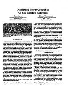
Autoregressive model of power control.

power that can be handled by the mobile station, and Γi (t) is the SINR of user i at time slot t, which is given by Γi (t) =

Pi (t)Gii (t) Q  j=1 j
=i

,

i = 1, . . . , Q

(4)

Pj (t)Gij (t) + δ(t)

i=1 t=1

where γ is an adaptation factor (also called forgetting factor) and N is the number of time slots in the time window. If the forgetting factor is not zero, then it means that the next transmitted power will depend on all the accumulated past history of the transmitted powers. Suppose further that power Pi (t) is described by an autoregressive model, as shown in Fig. 2 [17]. The transmitted power can be given as n 

wi (k)Pi (t − k) = wi Xi (t)

In practice, the transmitter power is bounded above by some maximum value Pmax determined by the properties of the power amplifier of the handset. It is interesting to observe that if λi,1 > 0, then the transmitted power of the MODPC algorithm (7) is naturally upper bounded such as Pi (t) < Pmin +

λi,2 sup Γ = Psup , λi,1 i

i = 1, . . . , Q.

(8)

Thus, we can conclude that Pmax ≥ Psup , i.e., the power constraint cannot be violated, as long as

where Gij (t) is the channel gain between user j and receiver i, Q is the number of active users at time slot t, and δ(t) is the average additive noise power at time slot t. Without loss of generality, it has been assumed that user i is assigned to base station i. We assume that the transmitted data of user i is correctly decoded at the receiver if the received SINR is greater than some minimum value Γi,min . An interpretation for the supremum SINR is that it is the minimum tolerable SINR determined by the utilized coding and modulation scheme + SINR margin to cope with fast fading. The obtained power control from minimizing the error function (3) is able to track the supremum SINR and with a penalty of using a large power. The error function (3) can be extended to include other objectives such as maximizing the throughput [16]. To generalize the optimization over all users for time window of N slots, we define the following optimization problem: Find the power vector P = [P1 , P2 , . . . , PQ ] (P denotes the transpose of vector P) that minimizes of the following cost function:  Q N  N −t 2 γ ei (t) , t = 1, . . . , N (5) J(P) =

Pi (t) =

t = 1, 2, . . . . (7)

(6)

k=1

where wi = [wi (1), . . . , wi (n)] is the power adaptation weight vector, Xi (t) = [Pi (t − 1), . . . , Pi (t − n)] contains known old values of the transmitted power, and n is the number of

λi,2 Pmax − Pmin ≤ λi,1 Γsup i

(9)

Since λi,2 = 1 − λi,1 , the preceding equation can be written in terms of λi,1 as λi,1 ≥

Γsup i

Γsup i . + Pmax − Pmin

(10)

In the general case, we need to augment the MODPC algorithm to take the maximum power constraint into account as follows:

 λi,1 Pmin + λi,2 Γsup i Pi (t − 1) Pi (t) = min Pmax , λi,1 Pi (t − 1) + λi,2 Γi (t − 1) i = 1, . . . , Q;

t = 1, 2, . . . . (11)

Some interesting observations of the MODPC algorithm (7) are that the MODPC algorithm is a nonlinear algorithm. Its behavior is determined by the values of the tradeoff factors λi . It requires no extra measurements other than those used in conventional algorithms [1]–[10]. At λi,1 = 0 and λi,2 = 1 − λi,1 = 1, the first objective in (3) is relaxed, and only the second objective is considered. It is interesting to observe that in this case, the MODPC algorithm becomes the very well known DPC algorithm [1], which is Pi (t) =

Γsup i Pi (t − 1). Γi (t − 1)

(12)

Hence, we note that the DPC algorithm is a special case of the MODPC algorithm. At the other extreme case where λi,1 = 1 and λi,2 = 0, the handset transmits at the minimum power, regardless of the SINR situation (i.e., no power control). The proper values of tradeoff factors, which could be adaptive, can greatly enhance the performance of the algorithm, depending on the scenario. In terms of MO optimization, the proper values of the tradeoff factors for a certain network situation are selected by the decision maker, who determines the optimum point from a Pareto

782

IEEE TRANSACTIONS ON VEHICULAR TECHNOLOGY, VOL. 56, NO. 2, MARCH 2007

optimal set. A simple but efficient decision rule can be derived from the steady-state behavior of the proposed algorithm: At steady state (i.e., Pi (t + 1) = Pi (t) = Piss ), (7) results in the steady-state SINR of user i(Γss i ), which is given by sup Γss − i = Γi

λi,1 (P ss − Pmin ) λi,2 i

(13)

Pmax , Pmax +Γsup i −Γi,min

λi,1 =

Γsup i −Γi,min . Pmax +Γsup i −Γi,min (14)

Let us consider the DS-CDMA case, where the relationship between the target SINR and the target Eb /I0 is given (in decibel scale) by ˆ sup = ρsup − Ω Γ i i

µ∗ = max min Γi . P≥0 i=1,...,Q

when λi,2 > 0. The case in which λi,2 = 0 denotes fixed transmission powers, and its steady-state analysis is omitted as trivial. One of the key features of the MODPC algorithm can be observed in the steady-state solution given in (13). It is clear that the steady-state SINR equals the supremum SINR when the steady-state power equals the minimum power. The penalty of using any excessive power is a reduction in steady-state SINR. This could be interpreted as dynamically changing SINR margin. If the system is lightly loaded, a large margin could be used, and when the load increases, the SINR margin is decreased to include more users. This behavior of MODPC resembles the gradual removal concept suggested by Yates et al. [22]. The decision maker should choose the tradeoff factors λi,1 and λi,2 so that all users can achieve at least the minimum acceptable SINR level. In the worst-case situation, the steadystate power is the maximum allowed power Pmax , which is determined by the power amplifier of the handset. A robust way to find the tradeoff factors values is to consider the worst case Piss = Pmax . It should be noted that proposing the tradeoff factors by this method is not necessarily optimum but gives an initial guess. From (13) and λi,1 + λi,2 = 1, the values of tradeoff factors can now be solved to yield (assuming Pmin = 0) λi,2 =

Definition 1: The network configuration is said to be “feasible” if there exists a power vector P∗ ∈ {P : 0 ≤ P ≤ Pmax } such that Γi ≥ Γi,min , i = 1, . . . , Q. Definition 2: The maximum achievable SINR µ∗ is defined as

(15)

where ρsup is the supremum bit-energy-to-noise-poweri spectral-density ratio in decibels and Ω is the processing gain = in decibels. As typical values in voice applications, ρsup i ˆ sup = −18 dB. If the margin 6 dB, Ω = 24 dB, and then Γ i is 3 dB and Pmax = 1, then from (14), λi,1 ∼ = 0.01, and 0.99. As stated before, the system designer decides λi,2 ∼ = the optimum values of the tradeoff factors based on targeted objectives. The tradeoff factors can be adapted to achieve certain time-varying objectives. The convergence properties of the MODPC algorithm are discussed in Section III. III. C ONVERGENCE A NALYSIS OF THE MODPC A LGORITHM Before proceeding to the convergence analysis, we consider the following definitions:

(16)

The convergence analysis of the MODPC algorithm is discussed in the next propositions. Proposition 1: For static channels and for any P (0) > 0, the MODPC algorithm (7) converges to a unique fixed point. This fixed point is determined by the values of the tradeoff factors explained in the previous section. The proof is given in Appendix III. Proposition 2: For a noiseless feasible system, static channels with P (0) > 0, and proper values of tradeoff factors, the MODPC algorithm converges to the SINR balance, i.e., lim P(t) = P∗

t→∞

lim Γi (t) = µ∗

t→∞

∀i = 1, 2, . . . , Q

(17)

where µ∗ is the maximum achievable SINR, and P∗ is the corresponding eigenvector of the normalized channel gain matrix F = [fij ], fij = Gij /Gii for i = j and fii = 0∀i [2]. See Appendix IV for the proof. IV. MODPC A LGORITHM W ITH Q UANTIZED SINR Perfect estimation of the mobile’s SINR at the base station is assumed in the MODPC algorithm. In the existing cellular communication system, only a quantized version of the SINR is available at the mobile station. In the worst case, only a 1-bit quantizer is used to command the mobile to step up/down its transmitted power. An estimation method for the SINR based on the 1-bit command is presented in [11]. In this section, we join this estimation method with the MODPC algorithm to see the quantization error effects on the algorithm. It can be shown from [11] than the estimated SINR at the mobile station is given by  t−1  sup ˜ i (t) = Γ − δi νi (t − k)ci (t, k) + νi (t) Γ k=1

t = 0, 1, . . . ; νi (t)

= sign (Γsup i

ci (t, k) =

i = 1, . . . , Q

− Γi (t)) EPC,i (t)

k−1 1 [1 + νi (t − n)νi (t − n − 1)] 2k n=0

(18) (19) (20)

where EPC,i (t) is 1 with probability PPCE,i (t) and −1 with probability 1 − PPCE,i (t). PPCE,i (t) is the probability of bit error in power control command transmission at time t. The same MODPC algorithm can be used with estimated SINR given in (18) as with perfect SINR. We call the new algorithm as MO totally DPC (MOTDPC) algorithm. The convergence property of the MOTDPC algorithm is discussed in the next corollary.

ELMUSRATI et al.: MODPC ALGORITHM FOR CDMA WIRELESS COMMUNICATION SYSTEMS

783

TABLE I AVERAGE TRANSMITTED POWER IN DECIBEL METERS

Corollary 1: For static channels and for any P (0) > 0, the MOTDPC algorithm converges to a unique fixed point. The proof is given in Appendix V. V. N UMERICAL R ESULTS In this section, we compare the convergence properties MODPC with DPC [1], Foschini’s and Miljanic’s algorithm (FMA) [6], and the second-order power control (SOPC) algorithm [10]. We compare the algorithms in terms of convergence speed, outage probability, and power consumption. The comparisons are carried out for both static and dynamic channels. In each channel scenario, we assumed 120 users uniformly distributed in an area of 4 km2 with four base stations. The base stations are regularly distributed, i.e., at (0.5,0.5), (0.5,1.5), (1.5,0.5), and (1.5,1.5) km. Perfect handover is assumed, where each user is assigned to the base station with the best instantaneous link quality. The maximum transmit power is normalized to 30 dBm. An additive white Gaussian noise is assumed with zero mean and an average power of −90 dBm. The radio link gain is modeled as a product of three variables: 1) the largescale propagation loss that depends on the distance between the mobile terminal and the base station; 2) lognormal shadowing with a mean of 0 dB and a standard deviation of 5 dB; and 3) Rayleigh-distributed multipath fading generated by a correlated process [20]. In the dynamic scenario, the speed of the users is 30 km/h. The carrier frequency is 2 GHz. In the snapshot analysis, the channel gain of each user is set at a fixed value during the simulation. The tradeoff factors for the MODPC algorithm has been set for all users to λi,1 = 0.01 and λi,2 = 0.99. In the dynamic scenario, the same values of the tradeoff factors are used. The algorithms are compared in terms of the error norm and the outage percentage. The error is defined as the difference between the actual transmitted power vector generated by the power control algorithm and the optimum power vector. The optimum power vector is the solution of the centralized power control algorithm. The outage is the percentage of users that do not achieve the minimum tolerable SINR level. We follow the approach taken, e.g., in [10], and consider outage in each time slot instead of just observing the steady-state behavior. The supremum SINR is set to −18 dB for all users. Note that SINR here denotes the SINR before dispreading. The minimum allowed SINR has been set to 3 dB lower than the supremum SINR. For comparison purposes, Table I lists the average transmitted power of all users in decibel meters of each power control algorithm for static and dynamic scenarios. Fig. 3 shows the convergence behavior of the MODPC and DPC algorithms for two users. The figure depicts that the power path trajectory of the MODPC algorithm is converging much

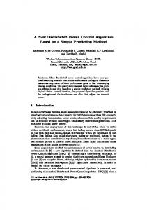
Fig. 3. Power path trajectories of two users using DPC and MODPC.

Fig. 4. Power convergence differences in DPC and MODPC.

faster toward the fixed point than that of the DPC algorithm. It is clear that the MODPC algorithm converges faster than the DPC algorithm to reach the feasible region. The MODPC algorithm requires less number of iterations than other conventional algorithms to converge to the adequate solution. It can be explained, as indicated by (3) and (13), that there is a penalty in using the power. Fig. 3 illustrates this property of the MODPC algorithm. The convergence analysis in [18] showed that the Hessian matrix associated with the MODPC scheme had a smaller spectral radius than the corresponding matrix for DPC. This result indicates that MODPC converges asymptotically faster than DPC. This observation is also supported by our simulation results here. It is, however, notable that the two algorithms are not converging to the same point. While DPC is converging toward Γsup i , MODPC is aiming to some lower SINR between Γi,min and Γsup i . This difference is clarified in Fig. 4. Fig. 4 shows the initial powers for both algorithms at point (1); then, MODPC converges to point (2), while DPC converges to point (3), which achieves Γsup i .

784

IEEE TRANSACTIONS ON VEHICULAR TECHNOLOGY, VOL. 56, NO. 2, MARCH 2007

Fig. 5. Comparison between different power control algorithms in terms of error and outage for the static-channel scenario.

Fig. 7. Comparison between different power control algorithms in terms of error and outage for the dynamic-channel scenario.

Fig. 6. Achieved SINR (in decibels) for the best and worst users. Fig. 8. Transmitted power versus time slots of different power control algorithms.

Fig. 5 shows comparisons of the error norm of the average outage percentage for the 120 users using MODPC, DPC, FMA, and SOPC algorithms for the static-channel case. It is clear in this scenario that the MODPC algorithm outperforms other algorithms in terms of power convergence speed and outage convergence speed. Moreover, the average consumption power of the MODPC algorithm is considerably less than those of other simulated algorithms, as indicated by Table I. For example, the average transmitted power of MODPC is lower than that of DPC by less than 4 dB. That means less than half of the power (on the average) is needed for the MODPC algorithm to achieve the target QoS. Comparing the MODPC algorithm with other algorithms, it is clear that less power is consumed by the MODPC algorithm. Fig. 6 shows the achieved SINR for the best and worst users using the MODPC algorithm. It is clear that the aim is to be in the convergence region between Γi,min and Γsup i . Dynamical channels with fast and slow fading are assumed in the second scenario. In this scenario, the comparison results

are quite similar in their trend as in the first scenario, as shown in Fig. 7. The MODPC still outperforms the other algorithms in terms of optimum power tracking capability in terms of error norm and QoS tracing capability in terms of outage. The average power consumption of MODPC is less than that of other algorithms, as shown in Table I. Since this scenario is for a dynamic channel, it is worth investigating the fluctuations of the transmitted power of one user and how the algorithms can track the optimum power. Fig. 8 depicts a sample of the transmitted power of an arbitrarily selected user using optimal (centralized), DPC, FMA, and MODPC algorithms. The result SOPC algorithm is omitted to enhance the visibility of the graphs because it contains high overshoots (the transmitted power falls close to zero at iteration 19). Fig. 8 indicates that the MODPC algorithm can track the variations of the channel better than other simulated algorithms. This result indicates that the MODPC algorithm can react faster to changes in interference than the other algorithms. Finally, the convergence

ELMUSRATI et al.: MODPC ALGORITHM FOR CDMA WIRELESS COMMUNICATION SYSTEMS

785

The error function can be modified such as ˆ i,2 (t) (Γi (t) − Γsup ) ei (t) = λi,1 (Pi (t) − Pmin ) + λ t = 0, 1, . . .

(21)

ˆ i,2 (t) = sign(Γi (t) − Γsup )λi,2 ; the sign function is where λ defined as

+1, x ≥ 0 (22) sign(x) = −1, x < 0. Suppose further that power Pi (t) is described by a linear autoregressive model, as shown in Fig. 2 [17]. The transmitted power is Pi (t) =

n 

wi (k)Pi (t − k) = w i Xi (t),

t = 0, 1, . . .

k=1

Fig. 9. Convergence behavior in terms of error norm and outage for MOTDPC with different power control command error levels.

behavior of the MOTDPC with estimated SINR and different power control command errors is shown in Fig. 9. The figure indicates that MOTDPC achieves close to ideal performance even if 1-bit feedback is used instead of perfect SINR values. The performance remains tolerable even with up to 20% power control bit error rate.

VI. C ONCLUSION In this paper, we suggested a novel DPC algorithm that is based on the MO optimization method. We considered two objectives: 1) QoS in terms of SINR and 2) power consumption. It should be noted, however, that the suggested power control scheme could be easily extended to take other objectives, such as throughput, into account. The algorithm is parameterized so that the designer can make a tradeoff between QoS and power consumption. A simple guideline is provided for the choice of these parameters such that the given QoS constraints can be met. In a snapshot case, the algorithm was proven to converge, starting from an arbitrary initial value. The simulation results indicated that the suggested MODPC algorithm outperformed the DPC, FMA, and SOPC algorithms in convergence speed and was able to track the QoS target better in the case of a fading channel. The proposed algorithm has also been modified to adopt estimated SINR (based on the up/down power control command) instead of the ideal values. The modified method is called the MOTDPC algorithm. It has been proven that in the snapshot case, the power vector sequence generated by the MOTDPC algorithm converges, starting from an arbitrary initial value. The simulations show that the MOTDPC converges even in case of power control command errors.

The absolute function of the first term in (3) is not needed because the transmitted power cannot be less than the minimum.

 Xi (t) = Pi (t − 1) · · · Pi (t − n) . (24)

Observe that Xi (t) contains known measured values of the transmitted power. Substitute (23) into (21) and (4). Then, error ei (t) can be written as   ei (t) = λi,1 w i Xi (t) − Pmin    ˆ i,2 (t) Gii (t)w i Xi (t) − Γsup . (25) +λ Ii (t) Denote

  ˆ i,2 (t) Gii (t) . αt := λi,1 + λ Ii (t)

(26)

Using this in (25), ei (t) becomes ˆ i,2 (t)Γsup . ei (t) = αt w i Xi (t) − λi,1 Pmin − λ

(27)

From (5) and (25), a necessary condition for the minimum is given as follows for all i = 1, . . . , Q: 2

N  t=1

γ N −t ei (t)

∂ei (t) = 0. ∂w

(28)

From (27) ∂ei (t) = αt X i (t). ∂w

(29)

Substituting (27) and (29) into (28), we obtain N 

γ N −t ei (t)

t=1

A PPENDIX I D ERIVATION OF MODPC A LGORITHM

(23)

where

 wi = wi (1) · · · wi (n) ,

=

N 

∂ei (t) ∂w

γ N −t (αt w i Xi (t) − λi,1 Pmin − λi,2 Γsup ) αt X i (t)

t=1

= 0.

(30)

786

IEEE TRANSACTIONS ON VEHICULAR TECHNOLOGY, VOL. 56, NO. 2, MARCH 2007

ˆ i,2 (t) To overcome these problems, only the positive values of λ ˆ are considered, i.e., λi,2 (t) = λi,2 . This simplification has considerably reduced the complexity of the MODPC algorithm with the price of slight degradation in the convergence speed. The MODPC algorithm becomes

Solving for wi 



N  

 γ N −t αt2 Xi (t)X i (t) wi

t=1

=

N 

γ N −t αt (λi,1 Pmin + λi,2 Γsup ) Xi (t)

(31)

t=1

or wi (N ) = R−1 xx (N )Rx (N ),

i = 1, . . . , Q

Pi (t) =

λi,1 Pmin + λi,2 Γsup Pi (t − 1) λi,1 Pi (t − 1) + λi,2 Γi (t − 1) i = 1, . . . , Q; t = 1, 2, . . . . (40)

(32) A PPENDIX II I MPORTANT T HEORIES FOR C ONVERGENCE A NALYSIS

where Rxx (N ) :=

N 

γ N −t αt2 Xi (t)X i (t)

(33)

  γ N −t αt λi,1 Pmin + λi,2 Γsup Xi (t).

(34)

t=1

Rx (N ) :=

N 

In this Appendix, we introduce the definition of the standard power control algorithm as well as the two theorems related to it, as given in [19]. The transmitted power of user i can be described mathematically as

t=1

Pi (t) = Ψi (P(t − 1), Γi (t))

Equations (32)–(34) are well known from least squares techniques. Equation (32) can be solved using the Recursive Least Square method. To avoid the matrix inversion, Rxx (N ) may be computed recursively as

(41)

(35)

where Ψ(•) is the interference function, and Γi (t) is the SINR of user i at time slot t. The interference function Ψ(•) is called “standard” when the following properties are satisfied for all nonnegative power vector P [19]:

Since the inverse of Rxx (N ) is needed, we can use the matrix inverse lemma to obtain [21]  1 −1 Rxx (N ) = R−1 xx (N − 1) γ 2  −1 R−1 xx (N − 1)αN Xi (N )X i (N )Rxx (N − 1) . (36) − 2 X (N )R−1 (N − 1)X (N ) γ + αN i i xx

• positivity, i.e., Ψi (P(t), Γi (t)) > 0; • monotonicity, i.e., if P ≥ P , then Ψi (P(t), Γi (t)) ≥ Ψi (P i (t), Γi (t)) > 0; • scalability, i.e., for all α > 1, αΨi (P(t), Γi (t)) > Ψi (αP(t), Γi (t)). A power control algorithm of form (38) is called standard if the utilized mapping Ψ(•) is the standard interference function. Standard power control algorithms have the two following properties.

In addition, Rx (N ) can be computed recursively as   Rx (N ) = γRx (N − 1) + αN λi,1 Pmin + λi,2 Γsup Xi (N ). (37)

Theorem 1 [19, Th. 1]

The power control algorithm is easy to implement and is also computationally light to be applicable for existing wireless communication systems. Next, the simplest case, where n = 1 in (23) and γ = 0, is considered. Solving (32), we obtain

Theorem 2 [19, Th. 2]

2 Rxx (N ) = γRxx (N − 1) + αN Xi (N )X i (N ).

wi (t) =

ˆ i,2 (t)Γsup λi,1 Pmin + λ ˆ i,2 (t)Γi (t − 1) λi,1 Pi (t − 1) + λ i = 1, . . . , Q;

ˆ i,2 (t)Γsup λi,1 Pmin + λ P (t − 1) ˆ i,2 (t)Γi (t − 1) i λi,1 Pi (t − 1) + λ i = 1, . . . , Q;

If Ψ(•) is feasible, then for any initial power vector P o , the standard power control algorithm converges to a unique fixed point P∗ .

t = 1, 2, . . . . (38)

From (23), the transmitted power of user i at time slot t is given by Pi (t) =

For a standard power control algorithm, solution of (41) has a unique fixed point.

t = 1, 2, . . . . (39)

ˆ i,2 (t) sign, the transmitted Due to the sharp changes in the λ power in (39) may take negative values as well as very large power values, which are not part of the power feasible subspace.

A PPENDIX III P ROOF OF P ROPOSITION 1 We will prove that the MODPC algorithm is a standard power control algorithm discussed in Appendix II; then, by Theorems 1 and 2, the MODPC algorithm converges to a unique fixed point. The interference function Ψi (P) of the MODPC algorithm is given by Ψi (P) =

λi,1 Pmin + λi,2 Γsup i Pi (t − 1) λi,1 Pi (t − 1) + λi,2 Γi (t − 1) i = 1, . . . , Q (42)

ELMUSRATI et al.: MODPC ALGORITHM FOR CDMA WIRELESS COMMUNICATION SYSTEMS

From (44), one can say that Ii (αP) > Ii (P), α > 1; then

and it can be represented as Ψi (P) =

Ii (P)a λi,1 Ii (P) + λi,2

Q  Gij (t)Pj (t) j=1 j
=i

Gii (t)

δ(t) Gii (t)

+

(44)

and a = λi,1 Pmin + λi,2 Γsup > 0. Note that for convenience, i the time symbol t has been omitted from the interference function as well as the normalized interference [e.g., use Ii (P) instead of Ii (P(t))]. From (44), it is clear that for any P ≥ 0,

Ii (P) ≥ 0.

αΨ(P) >

(43)

where Ii (P) is the normalized interference for user i such as Ii (P) =

787

(45)

P ≥ Z ⇒ Ii (P) ≥ Ii (Z).

A PPENDIX IV P ROOF OF P ROPOSITION 2 In (7), let a = λi,1 Pmin +λi,2 Γsup i . Since Γi (t) = Pi (t)/Ii (t), where Ii (t) is the normalized interference (44) with δ(t) = 0, (7) can be rewritten as

(46)

Since 0 ≤ λi,1 ≤ 1; λi,2 = 1 − λi,1 and from (43) and (45), then for any P ≥ 0 ⇒ Ψ(P) ≥ 0.

(47)

Thus, the “positivity” condition has been proven. The monotonicity condition will be proven by contradiction. For any P ≥ Z, assume that Ψi (P) < Ψi (Z). Then, from (43) Ii (P)a Ii (Z)a < (48) λi,1 Ii (P) + λi,2 λi,1 Ii (Z) + λi,2 

Ii (Z)a λi,1 Ii (P) + λi,2 Ii (P)a < (49) λi,1 Ii (Z) + λi,2   (Z) λi,1 Ii (Z) + λi,2 IIii(P) Ii (P)a < Ii (P)a . (50) λi,1 Ii (Z) + λi,2 However, from (46)  0