1 Finite volume schemes. 2 VFRoe numerical flux. 3 Solving the linearized Riemann problem. 4 Entropy fix. 5 Numerical results. Helluy Hérard Mathis Müller.
Finite volume schemes VFRoe numerical flux Solving the linearized Riemann problem Entropy fix Numerical results
A simple entropy fix for the VFRoe schemes P. Helluy1
J.-M. Hérard2 1 Université
H. Mathis1
S.Müller3
de Strasbourg
2 EDF 3 RWTH
Paris Aachen
Fourth workshop "Micro-Macro Modelling and Simulation of Liquid-Vapour Flows"
Helluy Hérard Mathis Müller
VRoe fix
Finite volume schemes VFRoe numerical flux Solving the linearized Riemann problem Entropy fix Numerical results
Outlines
1
Finite volume schemes
2
VFRoe numerical flux
3
Solving the linearized Riemann problem
4
Entropy fix
5
Numerical results
Helluy Hérard Mathis Müller
VRoe fix
Finite volume schemes VFRoe numerical flux Solving the linearized Riemann problem Entropy fix Numerical results
Finite volumes Approximation of ∂t W + ∂x F (W ) = 0 + entropy condition Mesh xi = i∆x, tn = n∆t,Win ' W (xi , tn ) Finite volume approach n n Win+1 − Win Fi+1/2 − Fi−1/2 + =0 ∆t ∆x
Numerical flux n n Fi+1/2 = F (Win , Wi+1 )
Conservative variables W (Y ) and primitive variables Y ∂t Y + A(Y )∂x Y = 0 Helluy Hérard Mathis Müller
VRoe fix
Finite volume schemes VFRoe numerical flux Solving the linearized Riemann problem Entropy fix Numerical results
Example: Rusanov scheme
The numerical flux of the Rusanov scheme is given by F (WL , WR ) =
F (WL ) + F (WR ) λ − (WR − WL ) 2 2
where λ = max (ρ(A(YL )), ρ(A(YR )) The Rusanov scheme generally satisfies a numerical entropy dissipation principle. It is robust but very dissipative.
Helluy Hérard Mathis Müller
VRoe fix
Finite volume schemes VFRoe numerical flux Solving the linearized Riemann problem Entropy fix Numerical results
VFRoe approach solve the linearized Riemann problem ∂t Y + A(Y )∂x Y = 0 � YL + YR YL if x < 0, Y (x, 0) = Y= YR if x > 0. 2 The solution is noted Y (x, t) = R(YL , YR , x/t) The numerical flux of the VFRoe scheme is then F (WL , WR ) = F (R(YL , YR , 0)) Helluy Hérard Mathis Müller
VRoe fix
Finite volume schemes VFRoe numerical flux Solving the linearized Riemann problem Entropy fix Numerical results
Linearized Riemann problem
The solution of the linearized Riemann problem is given by Y (x, t) = R(YL , YR , x/t) = with
x YL + YR 1 − sgn(A(Y ) − I )(YR − YL ) 2 2 t
1 if x > 0, 0 if x = 0, sgn(x) = −1 if x < 0.
Helluy Hérard Mathis Müller
VRoe fix
Finite volume schemes VFRoe numerical flux Solving the linearized Riemann problem Entropy fix Numerical results
The sgn function of the matrix A can be defined as follow. Let λ1 < λ2 < · · · < λm be the ordered eigenvalues of A. Let P be the interpolation polynomial of the sgn function on the eigenvalues of A: d ◦P ≤ m − 1 P(λi ) = sgn(λi ) i = 1 · · · m Then sgn(A) := P(A)
Helluy Hérard Mathis Müller
VRoe fix
Finite volume schemes VFRoe numerical flux Solving the linearized Riemann problem Entropy fix Numerical results
An efficient way to compute P is to use the Newton algorithm P(A) = sgn[λ1 ] + sgn [λ1 , λ2 ] (A − λ1 I) + · · · +sgn [λ1 · · · λm ] (A − λ1 I ) · · · (A − λm−1 I ) sgn[λi ] := sgn(λi ) sgn [λ1 · · · λi+1 ] =
sgn [λ2 · · · λi+1 ] − sgn [λ1 · · · λi ] λi+1 − λ1
easy to handle the case of multiple eigenvalues (away from 0) the computation of the eigenvectors is not necessary complexity equivalent to the Hörner algorithm (∼ m − 1 matrix vector products)
Helluy Hérard Mathis Müller
VRoe fix
Finite volume schemes VFRoe numerical flux Solving the linearized Riemann problem Entropy fix Numerical results
A simple entropy fix
The precision of the VFRoe scheme is equivalent to the precision of the Godunov or the Roe scheme. The choice of the primitive variables is important (and problem dependant) [2] The cost and simplicity are very interesting (∼Rusanov + 15%) But an entropy fix is needed in sonic waves
Helluy Hérard Mathis Müller
VRoe fix
Finite volume schemes VFRoe numerical flux Solving the linearized Riemann problem Entropy fix Numerical results
We propose to follow the very simple idea: replace the VFRoe flux by the Rusanov flux if a sonic wave is present. More precisely, if for a genuinely non-linear field we have λi (WL ) < 0 < λ (WR ) then replace the VFRoe flux by the Rusanov flux. No small parameter as for other entropy fix fast It is not clear why it should work: numerical tests for the moment...
Helluy Hérard Mathis Müller
VRoe fix
Finite volume schemes VFRoe numerical flux Solving the linearized Riemann problem Entropy fix Numerical results
Numerical results We first consider a Riemann problem for the Euler system with a strong rarefaction wave W = (ρ, ρu,
p ρu 2 + ) γ −1 2
γpu ρu 3 + ) γ −1 2 p Y = (ρ, u, s = γ ) ρ
F (W ) = (ρu, ρu 2 + p,
γ = 1.4, CFL = 1/2, ρL = 0.01, uL = 0, pL = 5, ρR = 1000, uR = 0, pR = 105 The initial jump is at x = 1/2 Helluy Hérard Mathis Müller
VRoe fix
Finite volume schemes VFRoe numerical flux Solving the linearized Riemann problem Entropy fix Numerical results
Density 1000
800
600
400
200
0
0
0,2
0,4
0,6
0,8
Helluy Hérard Mathis Müller
VRoe fix
1
Finite volume schemes VFRoe numerical flux Solving the linearized Riemann problem Entropy fix Numerical results
Density (zoom) 0,2
0,15
0,1
0,05
0
0,02
0,04
0,08
0,06
Density profiles obtained by using 500 cells (circles), 1000 cells (dashes), 5000 cells (dotted), 10000$ cells (plain). Helluy Hérard Mathis Müller
VRoe fix
Finite volume schemes VFRoe numerical flux Solving the linearized Riemann problem Entropy fix Numerical results
Magnetohydrodynamics The MHD equations with divergence cleaning [3] read W = (ρ, ρu T , u = (u1 , u2 , u3 )T ,
p ρu · u + B · B T + , B , ψ)T γ −1 2 B = (B1 , B2 , B3 )T ,
n = (1, 0, 0)T
ρu · n ρ(u · n)u + (p + B·B 2 )n − (B · n)B γp ρu·u ( + + B · B)u · n − (B · u)(B · n) F (W ) = γ−1 2 (u · n)B − (B · n)u + ψn ch2 B · n Y = (ρ, u T , p, B T , ψ)T Helluy Hérard Mathis Müller
VRoe fix
Finite volume schemes VFRoe numerical flux Solving the linearized Riemann problem Entropy fix Numerical results
ρL = 3, uL = (1.3, 0, 0)T , pL = 3, BL = (1.5, 1, 1)T , ψL = 0 ρR = 1, uR = (1.3, 0, 0)T , pR = 1, BR = (1.5, cos(1.5), sin(1.5))T , ψR = 0 CFL = 0.8, x ∈ [−1; 6]. ch = 3.8 γ = 5/3 The initial jump is at x = 0 We take 2000 cells
Helluy Hérard Mathis Müller
VRoe fix
Finite volume schemes VFRoe numerical flux Solving the linearized Riemann problem Entropy fix Numerical results
Density 3 rho ’rho_vfroe’ ’rho_vfroe_fixed’ ’rho_rusanov’
2.5
2
1.5
1 -1
0
1
2
3
Helluy Hérard Mathis Müller
4
VRoe fix
5
6
Finite volume schemes VFRoe numerical flux Solving the linearized Riemann problem Entropy fix Numerical results
Magnetic field B2 1 B2 ’B2_vfroe’ ’B2_vfroe_fixed’ ’B2_rusanov’
0.9 0.8 0.7 0.6 0.5 0.4 0.3 0.2 0.1 0 -1
0
1
2
3
Helluy Hérard Mathis Müller
4
VRoe fix
5
6
Finite volume schemes VFRoe numerical flux Solving the linearized Riemann problem Entropy fix Numerical results
C. Altmann, T. Belat, M. Gutnic, P.Helluy, H. Mathis, Galerkin discontinuous approximation of the magneto-hydrodynamics equations, INRIA report, 2008. T.Buffard, T. Gallouët, J.M. Hérard, A sequel to a rough Godunov scheme. Application to real gases, Computers and Fluids, vol. 29, pp. 813-847, 2000. A. Dedner, F. Kemm, D. Kröner, C.-D. Munz, T. Schnitzer, and M. Wesenberg. Hyperbolic divergence cleaning for the MHD equations. J. Comput. Phys., 175(2):645–673, 2002 P. Helluy, J.-M. Hérard, H. Mathis, S. Müller, A simple parameter-free entropy correction for approximate Riemann solvers, preprint, 2009.
Helluy Hérard Mathis Müller
VRoe fix