15 MAY 2000
HALL
1557
A Simple GCM Based on Dry Dynamics and Constant Forcing NICHOLAS M. J. HALL Department of Atmospheric and Oceanic Sciences, and Centre for Climate and Global Change Research, McGill University, Montreal, Quebec, Canada (Manuscript received 25 January 1999, in final form 8 July 1999) ABSTRACT A dry spectral primitive equation model is used to simulate the global atmospheric circulation during northern winter. The resolution is T21 in the horizontal, with five equally spaced sigma layers. The only additional terms in the equations are those describing linear damping, linear scale-selective diffusion, and time-independent forcing. The damping and diffusion act on temperature and momentum. The forcing acts on all prognostic variables. It is calculated objectively from the tendencies produced when the model is initialized with a long time series of observational analyses, and separated into components to ease comparison with time-dependent perturbation models. The simulated climate reproduces observed features of the circulation, both time-mean fields and transienteddy covariances, with remarkable success. The accurate simulation of tropical divergent flow is a particularly useful result. The main deficiencies are an underestimation of transient-eddy kinetic energy and a lack of transient activity in the Southern Hemisphere. In an attempt to reduce the forcing of divergent flow, a modified vertical scheme and modified forcing functions based on a calculation of balanced flow are introduced. The former still has significant divergence forcing and makes little difference to the final result. The latter tends to give solutions that are unrealistic in the Tropics. The model’s sensitivity to variations in forcing functions and damping parameters is further explored. The Southern Hemisphere transient behavior can be improved by boosting the local forcing of baroclinicity by up to a factor of 2, and a simulation of the Southern Hemisphere winter is relatively successful. The applications and limitations of such a simple fast-running climate model with a relatively realistic simulated climate are discussed.
1. Introduction There are a multitude of different approaches to modeling climate perturbations. Often the approaches are complementary. A comprehensive general circulation model (GCM) might simulate the observed climate realistically using principles that are as physically based as possible. This engenders a certain amount of confidence in the GCM’s ability to simulate perturbations to the climate, whether they arise from anomalous external forcing or internal variability. However, GCMs are typically very complicated, relying on physical parameterizations that can interact with one another and with the basic dynamics. Such interactions are often important, but they can be difficult to diagnose and the dominant process leading to a particular model response, if it exists, can be difficult to isolate. An alternative approach is to work with idealized models, which concentrate on a small number of pro-
Corresponding author address: Dr. Nicholas M. J. Hall, Department of Atmospheric and Oceanic Sciences, McGill University, 805 Sherbrooke St. W., Montreal, PQ H3A 2K6, Canada. E-mail:
[email protected]
q 2000 American Meteorological Society
cesses, often with reduced dimensionality, idealized domains, or simplified equations. They are computationally cheap and susceptible to rigorous analysis. They are an invaluable aid to understanding, but they usually sacrifice a certain level of realism. The territory between these two extremes is occupied by what is loosely described as ‘‘diagnostic modeling.’’ Data from observations or more comprehensive simulations are used to provide part of the solution, and the sensitivity to variations in forcing or model parameters can be explored in a controlled and relatively realistic setting. Linear stationary wave models, and perhaps some normal-mode life cycle experiments fall into this category. The drawback of this approach is that the solutions are usually constrained by the formulation of the model. Such models are often linearized about a climatology, time independent, or nonequilibrium initial value problems. Important interactions associated with finite amplitude transient perturbations are seldom treated correctly, if at all by these models. In this paper a method of extending this type of model toward the realism enjoyed by GCMs is explored. The objective is to develop a model that can be used to help identify the limits of dry dynamical processes in ac-
1558
JOURNAL OF THE ATMOSPHERIC SCIENCES
counting for the existence of climate anomalies seen in observations or in more comprehensive modeling studies. The resulting model can also be used for climate studies in its own right. The work is presented so that the link between this model and simpler models in the diagnostic class can be clearly seen. Starting with the dry spectral primitive equation model due to Hoskins and Simmons (1975, hereafter HS), time-independent forcing terms are calculated empirically from a long time series of observational analyses. These forcing terms represent an attempt to correct the systematic errors that would arise from integrating the dry dynamical equations alone to simulate the climate. It is to be hoped that they correspond to the long-term mean of the diabatic forcing that might come from physical processes in the atmosphere or the physical parameterizations in a GCM. The procedure followed is essentially the same as that used by Roads (1987) for a quasigeostrophic model and extended by Chen et al. (1993, hereafter CRA) to a stripped down GCM with a moist convection scheme. These two studies were concerned with predictability. The same method has been used in a quasigeostrophic model by Marshall and Molteni (1993) to study low-frequency variability and by Lin and Derome (1996) to study predictability. The extension of this method from the quasigeostrophic set to the primitive equations is not trivial. It is worthwhile, however, because it allows for a realistic simulation of divergent tropical flows, which is essential to many important climate phenomena. The model proposed in this paper is therefore perhaps the simplest prescription for a GCM that has a realistic climate over the whole globe but is based entirely on dry dynamics, time-independent forcing, and linear damping. This approach is equivalent to the ‘‘restoration forcing’’ used in previous studies with primitive equation models, in which the damping operator acts on the difference between the model state and some specified ‘‘equilibrium’’ state. Most of these studies have concentrated on the zonal-mean midlatitude flow, with a variety of objectives from testing the numerics (Held and Suarez 1994) and the role of resolution (Boer and Denis 1997) to lowfrequency variability studies (James and James 1989; Yu and Hartman 1993). In most cases the forcing strategy has grown out of a combination of experience and a desire for simplicity. In this study we assess the performance of a single-objective method. In section 2 the method of calculating the forcing terms will be described in detail. The problem of the dynamical balance in the primitive equations and the choice of variables to be forced will be faced. Section 3 gives a brief description of the model, the data analysis, and the experimental design. The results are displayed for various choices of forcing in section 4, and section 5 outlines the sensitivity of the model’s climate to a small number of damping parameters. Section 6 contains some discussion and conclusions. The casual reader may wish to skip sections 2b, 4b, and 5, which
VOLUME 57
contain results pertaining to the model’s sensitivity that should be of interest to researchers engaged in similar work. 2. Calculating the forcing a. Outline of the method A realistic simulation of a statistically steady climate should accurately reproduce its time-mean state. It should also possess variability that resembles in a statistical sense, the variability seen in a long time series of the observed climate, both in its temporal and spatial characteristics. In what follows it is assumed that this type of behavior is realizable in the model used, with the restriction that the forcing is time independent. Consider an observed atmospheric state, which is fully described by the state vector F. That is to say F is a vector of coefficients in some basis, which represents the instantaneous state of the atmosphere. The number of coefficients contained within F will depend on the resolution of the analysis and the number of field variables observed. The instantaneous time evolution of F is described by dF 5 N(F) 1 f (t), dt
(1)
where N is a nonlinear operator in the same basis as F. Here N can be defined so that it corresponds exactly to the unforced behavior of the model we wish to use. Whatever remains in the observed tendency defines f, the external forcing. The f is therefore independent of F but, in general, it is a function of time. In a perfect model f would be nothing more than a prescribed boundary forcing, and all other processes would be contained within N. However, we wish to prescribe N as the dry primitive equations plus some simple damping. Many of the internal interactions of the system (e.g., heating due to moisture condensation) will therefore be viewed as external forcing and added to f. Consider now a model whose instantaneous state is described by the vector of coefficients C, in the same basis as F. Our goal is to produce a simulation of Eq. (1) based on a model whose tendency is described by dC 5 N(C) 1 g, dt
(2)
where g is a constant vector. The problem is therefore one of specifying g so as to give the most realistic simulation of (1) with the constraint that g must be time independent. It would seem natural to set g equal to the long-term mean of f. In the remainder of this section we will examine this choice in more detail. The time-mean budget of (1) can be formed by splitting F into a long-term mean F and an instantaneous perturbation F9. Thus,
15 MAY 2000
1559
HALL
F 5 F 1 F9
and
dC 5 N(C) 1 E(C9) 1 g 5 0. dt
N(F) 5 N(F) 1 L(F9) 1 E(F9), where L is a linear operator (the linearization of the model N about the climatology F) and E is a nonlinear operator of the same degree as N but with no linear terms. Note that L and E depend on F. For a long time series from a statistically steady climate (i.e., a climate with no long-term trend) the time mean of (1) yields dF 5 N(F) 1 E(F9) 1 f 5 0. dt
(3)
If (3) did not equate to zero, but instead the left-hand side had a magnitude comparable to that of the individual terms on the right, there would be a large difference between the climate at the end of the time series and that at the beginning, and it would not be possible to model this system using (2). This is because we view (2) as an expression of a system in statistical equilibrium. An integration of (2) either reaches a statistical equilibrium or is unstable and unable to give useful solutions after a long time. The method is therefore not suitable for the simulation of an externally driven trend. This may be a concern if there is a very large-amplitude climate change in the observed time series. It compromises the applicability to the equinox seasons. In this paper we concentrate on the winter season, where the left-hand side of (3) is negligible compared to the other terms. Setting g 5 f gives g 5 2N(F) 2 E(F9) 5 2N(F).
(4)
A time-independent ‘‘diabatic’’ forcing is thus defined in terms of the action of the model operator N on observed atmospheric states F. Equation (4) splits this forcing into two components, 2N(F) and E(F9). The former, 2N(F), represents the maintenance of the timemean flow against its own advective tendencies and against damping. In the atmosphere, the processes that maintain the time-mean budget against these tendencies are diabatic forcing and transient-eddy flux convergence. The 2N(F) therefore represents the sum of these two effects. If we set g 5 2N(F), this would be the appropriate forcing for a model that had no explicit representation of transient-eddy fluxes. The second term, E(F9), is often dubbed the ‘‘transient-eddy forcing.’’ It represents the effect of observed transient fluxes on the time-mean budget. Since our intention is to build a model that deals explicitly with transient eddies, this term is subtracted from the first. If this is done, and g is specified as in (4), the model freely develops its own transient-eddy activity and g is a proxy for diabatic forcing alone. The time-mean budget equation for the model is obtained by taking the time-mean of a long integration of (2):
(5)
From (4) we obtain N(C) 1 E(C9) 5 N(F) 1 E(F9).
(6)
This equation defines the extent to which the model integration must resemble the data. The choice of forcing guarantees that the mean tendency in each variable calculated by the model before forcing is applied will equal the mean tendency the unforced model would predict if initialized with observed atmospheric states. If the dynamics are essentially advective, this is equivalent to saying that the mean flux convergence of each variable in the model is the same as its mean flux convergence in the observations. However, the mean flux convergence is made up from fluxes by the time-mean flow and fluxes by the transient eddies, corresponding the first and second terms on each side of (6). The balance between these two contributions is not guaranteed by (6) to be the same in the model as in the observations. This method of forcing therefore does not guarantee a realistic model climatology. It remains to outline the method for calculating g. The effect of N on any initial condition C 0 can be found by running the model without forcing for one time step, giving the instantaneous tendency
1 2 dC dt
5 N(C0 ) 5 unf
1 Cunf 2 C0 , dt
(7)
where the subscript unf denotes an unforced integration of the model and the superscript 1 refers to the state after one time step. The length of the time step is dt. Thus N(F) can be found by setting C 0 5 F, and N(F) can be found by averaging the results of setting C 0 5 F i , where subscript i identifies one realization of F among n observations. Thus g 5 2N(F) 5 2
1 nd t
O {C n
1 iunf
2 Fi},
(8)
i51
while N(F) 5
1 Cunf 2F dt
and
(9)
E(F9) 5 N(F) 2 N(F).
(10)
It is of some practical value to know the separate contributions to g given in (9) and (10). Since the operator E has no linear terms, and is independent of any linear terms in N, the linear damping used in the model can be changed without altering E(F9). The appropriate change to g can therefore be made without stepping through the entire time series of data, just by considering the change to N(F). The possibility also exists of integrating a companion perturbation model closely related to the simple GCM by setting the forcing equal to
1560
JOURNAL OF THE ATMOSPHERIC SCIENCES
g9 5 2N(F)
[5g 1 E(F9)].
(11)
As mentioned above, such a forcing would now include the effect of observed transient-eddy fluxes. If the model state is specified as C 5 F 1 C p , where C p is a small perturbation to the observed climatology, the model equation becomes dCp 5 L(Cp ), dt
(12)
the associated time-dependent linear perturbation model. This method has been used by Hall and Sardeshmukh (1998) to examine the first eigenmode of L, and by Jin and Hoskins (1995) to study the direct response to a perturbation in the forcing. If C p becomes large, (12) is no longer true, but the method shown in (11) can still be used for a limited time to study the effect of nonlinearities on the growth of perturbations. b. Comparison with a balanced system In a system where F contains only one field variable, (1) can be rewritten as a single dynamical equation in this variable, and its spatial and temporal derivatives. This is true for the quasigeostrophic system where ]q 5 2J(c, q) 2 R(c) 1 S. ]t Here c is the streamfunction; q is the potential vorticity, a linear elliptic function of c; R is a linear damping function; and S represents the constant forcing, in this case a source of potential vorticity. The evolution of the flow is determined by a single prognostic equation, and quantities such as temperature and divergence are merely functions of c. The two terms that define g in Eq. (4) have the following equivalents: 2N(F) 5 J( c , q ) 1 R( c )
and
E(F9) 5 2J(c 9, q9), where q and c are taken from observations. With suitable tuning of R, remarkably good simulations of the midlatitude atmosphere have been obtained by Roads (1987), Marshall and Molteni (1993), and Lin and Derome (1996). The balance of terms in (6) turns out to be very good, providing a realistic simulation of both the time-mean flow and the transient eddies. Is this just a happy coincidence? Does it derive from the balanced nature of the quasigeostrophic system? Can this result be repeated for the dry primitive equations? For the primitive equations the state vector F can be said to contain the fields of vorticity, divergence, temperature, and surface pressure (j, D, T and p* ). The primitive equations themselves can be written as four prognostic equations, one for each variable, and one diagnostic equation expressing hydrostatic balance (see HS for details specific to the model used here). In general, g will contain forcing terms for all four variables,
VOLUME 57
implying an explicit forcing of the divergent flow not present in the quasigeostrophic case. A state of balance might be defined as one where the tendency in the divergence equation is small, and the forcing of D makes a correspondingly small contribution to g. Such a state is not guaranteed by the primitive equations. However, on the timescales and space scales of interest to us, the atmosphere is close to such a balance, at least in midlatitudes. The parameterizations found in GCMs rarely provide a significant source of D, p* , or vertical velocity, even in the Tropics. It might therefore be of interest to seek a forcing that is consistent with this notion of balance, even though the primitive equations themselves cannot progress from one balanced state to another, and look at the consequences for the midlatitude flow, which is close to geostrophic, and the tropical flow, which has significant divergence. Consider first the part of the forcing, g, which is based on the time-mean flow [i.e., 2N(F)] and depends only on F. If we wish to remove the forcing of divergence from this term, and yet retain the definition of g given in (4), we must redefine F. Here F can be altered so that if it were used to initialize the unforced model [as in (9)] there would be no tendency in the divergence. Such solutions, F bal , can be found by an iterative procedure (see the appendix). There is no unique choice for F bal . We shall use the one in which D, T, and p* are unchanged but j is recalculated. Provided we can accept the redefinition of F as F bal , Eq. (6) still holds exactly. The application of the concept of balanced flow to the other part of the forcing, 2E(F), is more difficult. In principle one could construct solutions F ibal , which were close to each individual data realization F i , but the mean of the F ibal would not necessarily equal F bal . In practice such solutions prove difficult to find as the iteration scheme often fails to converge. A variation of the method used by CRA will be discussed briefly in section 4b. 3. Model and data The results shown in this paper come from the primitive equation model first developed by HS for the simulation of baroclinic wave life cycles (see, e.g., Simmons and Hoskins 1978). The version used here is almost identical to that of HS. It has spectral representation in the horizontal and a semi-implicit time step that is split so that diabatically induced tendencies (forcing, damping, and diffusion) are not passed through the semi-implicit scheme. The model uses sigma coordinates in the vertical and the vertical scheme conserves mass, energy, and angular momentum, based on the method of Simmons and Burridge (1981). Some results will also be shown for a modified version of this scheme designed to minimize the inferred divergence forcing. Details are given in the appendix. The model integrates equations for j, D, T, and log( p* ). In this study the
15 MAY 2000
HALL
resolution is set at T21 global domain, with five equally spaced sigma levels. Subgrid-scale dissipation is represented by scale-selective ¹ 8 hyperdiffusion, applied to j, D, and T throughout the atmosphere with a timescale of one day at the smallest scale. Additional linear damping is also applied to these fields uniformly in the horizontal and with a fixed vertical profile in the same manner as in Hall and Sardeshmukh (1998). On the lowest sigma level, j and D are damped with a timescale of one day and T with a timescale of two days. These timescales are chosen to represent the physical processes of boundary layer drag and surface exchange of sensible and latent heat, and are broadly consistent with budget studies such as that of Klinker and Sardeshmukh (1992). On other levels, 10-day damping is applied only to T. The effect of varying all these damping characteristics will be explored in section 5. The data used to derive the forcing fields are based on twice-daily global analyses from the European Centre for Medium-Range Weather Forecasts (ECMWF) Nine years (1980/81 to 1988/89) of winter (DJF) data are used. We take the first 90 days from each season (to aid calculation of time-filtered transients), resulting in a total of 1620 individual realizations. Horizontal velocity, temperature, and 1000-mb geopotential height on a 144 3 73 grid are linearly interpolated onto a highresolution 128 3 64 Gaussian grid to minimize horizontal interpolation errors. Orography is not represented explicitly in the model and surface pressure is calculated by integration of the barometric equation from the 1000mb height to zero using the 1000-mb temperature. In the remainder of the paper this quantity will be referred to as the mean sea level (MSL) pressure in both observations and model results. Other data provided on pressure surfaces are linearly interpolated onto the model’s sigma levels. The fields are then spectrally analyzed at T21 to give coefficients of j, D, T, and log( p* ). In sigma coordinates, the time-mean vertical integral of the continuity equation yields
E 1
0
D ds 5 2
1E 1
0
2
y ds · = logp*.
To take account of possible vertical interpolation errors, a correction is applied to D, which is independent of height and time, to ensure the above relation holds for the entire time series. The resulting climatology is shown in Fig. 1, which gives zonal-mean profiles of zonal and meridional wind, the jet structure at 300 mb, and the MSL pressure. Also shown are the high-pass filtered transient-eddy northward fluxes of temperature (900 mb) and eastward momentum (300 mb). The time filter used is the three-day block type employed by Hoskins et al. (1989), whereby high-pass quantities are defined according to
y 9T9HP 5 y 9T9 2 y 9T9, 3 3 where the subscript 3 refers to a dataset consisting of
1561
contiguous three-day means. This filter roughly isolates covariances with timescales less than six days. All integrations shown in the following sections are for 1000 days, starting with a resting atmosphere at a uniform temperature of 250 K. The first 300 days of these integrations are discarded, and the analysis is performed on the remaining 700. 4. Results a. Standard model and forcing If the unforced model is initialized with the timemean state displayed in Fig. 1, the model tendency is N(F). This is shown in Fig. 2 for the zonal means of the zonal and meridional winds, temperature, and MSL pressure. Note that if there were no advection, this tendency would not be zero as it also arises from the damping included in the definition of N. This is clear from the vertical profile of the temperature tendency, which basically displays a Newtonian cooling (to a uniform 250 K), particularly in the lowest layer where the timescale is shorter. Variations with longitude (not shown) display maxima over land in the Southern (summer) Hemisphere and minima over land in the Northern (winter) Hemisphere. The zonal wind has quite a small tendency, except at low levels where it is subject to stronger damping and at mid- to high latitudes in the Southern Hemisphere where there is a strong dipole structure aloft. Variations with longitude are quite strongly influenced by the need to balance the flow in the vicinity of orography. The tendency of the divergent flow is comparatively strong, as seen in both meridional wind and MSL pressure. The large-scale flow in the uppermost layer has a tendency to converge toward the equator. A corresponding migration of mass from mid- to low latitudes is apparent in the MSL pressure tendency. This feature is remarkably uniform in longitude. It can be attributed to a cancellation between two large terms in the divergence equation, one due to nonlinear contributions (such as advection) and the other due to the Laplacian of the geopotential. The latter term is very sensitive to the vertical scheme, and in the scheme adopted here the calculated geopotential is out of balance with the winds, leading to the large tendency seen in the divergence. This effect is also responsible for the large cooling that extrudes to high levels at midlatitudes. A version of the model with a modified vertical scheme designed to minimize this effect will be discussed in section 4b. As shown in section 2 [Eqs. (11) and (12)] if we now use 2N(F) to force the model, and it is initialized with the time-mean climatology, there should be no further development. However, if we initialize the model from a resting isothermal state, there is no guarantee it will attain the observed climatology or anything resembling it. In fact, when this is done and the spinup period is discarded, the model does produce a time-mean state
1562
JOURNAL OF THE ATMOSPHERIC SCIENCES
VOLUME 57
FIG. 1. The ECMWF 9-yr (1980/81 to 1988/89) winter (DJF) time-mean climatology. Negative contours dashed, zero contour dotted. (a) Section (latitude against sigma—Referenced to MSL pressure) of zonal-mean zonal wind; contours 5 m s 21 , negative regions shaded. (b) Section of zonal-mean meridional wind; contours 0.2 m s 21 , negative regions shaded. (c) 300-mb zonal wind; contours 8 m s21 . (d) MSL pressure, contours 6 mb. (e) High-pass filtered transient-eddy northward temperature flux; contours 3 K m s 21 , zero contour omitted. (f ) High-pass filtered transient-eddy momentum flux; contours 8 m 2 s22 , zero contour omitted.
identical to the observed climatology. Obviously, once it has reached such a state, there will be no time variation. This result merely tells us that for the damping parameters chosen, the observed climatology is stable. It is also likely to be the only stable state for this forcing, or at least the nearest one to a state of rest (note, however, that small changes in the damping or a change of resolution could remove this stability). What little transient activity we do see in these runs resembles a storm track mode, the slowest decaying one, as in Hall and Sardeshmukh (1998). Whitaker and Sardeshmukh
(1998) have shown that stochastic forcing of such modes in a stable system can give rise to a realistic transienteddy climatology. This experiment is a useful test of the model’s behavior with perturbation studies in mind, but in order to generate a model with realistic-amplitude eddies, it is clearly necessary to specify g as in (4) and allow the model to develop its own finite-amplitude transient eddies. Figure 3 displays E(F9) as calculated from the raw data [Eqs. (8), (9), and (10)]. It is displayed in the same way as N(F) was in Fig. 2, but note that the
15 MAY 2000
HALL
1563
FIG. 2. Zonal-mean single time step tendency N(F). Implied change per 1-h time step against latitude and pressure for (a) zonal wind, contours 0.05 m s21 ; (b) meridional wind, contours 0.2 m s21 ; (c) temperature, contours 0.1 K; negative contours dashed, zero contour dotted, negative regions shaded; and (d) MSL pressure, mb.
contour intervals are reduced in some cases because the amplitudes are lower. The transient eddies act to bolster the midlatitude westerlies at the downstream ends of the jets and to transfer heat poleward in the storm track entrance regions. There is also a forcing of divergence at upper levels in the midlatitudes and a corresponding movement of mass. The divergent part of the tendency is still relatively large, but smaller than the contribution from the time-mean flow. Having calculated the forcing term g using the method shown in (8), a long integration of the model can be performed. Figs. 4a,b shows some graphs of time-mean zonal mean quantities from the 9-yr observational analyses. Results from the model integration are shown for comparison in Figs. 4c,d. The first set of graphs in each case shows simple time-mean quantities and the second shows unfiltered transient-eddy products. Comparing simple time means, we see that the simulation gives a good account of the zonal-mean zonal jets at 300 mb with westerlies and easterlies at the right latitudes and with close to the right magnitude. At the same level the meridional wind gives an indication of the positions of the zonal-mean circulation cells. We see
that the Hadley cell and the Northern Hemisphere Ferrel cell are well simulated, but the model performs poorly in the Southern Hemisphere, where zonal-mean meridional circulation is much weaker than observed. The zonal-mean MSL pressure shows reasonable variation with latitude, except that it drops somewhat toward the North Pole, and the Southern Hemisphere has problems again as the surface westerlies are underestimated. In the Northern Hemisphere the total transient-eddy fluxes of temperature at low levels and momentum at upper levels are well simulated by the model in both position and magnitude. The total transient-eddy kinetic energy [EKE 5 0.5(u9 2 1 y 9 2 )], on the other hand, is only half of what it should be. To have accurate transient EKE is a severe test of any model, and many GCMs of higher resolution suffer from the same problem (see, e.g., Boville 1991). Increasing resolution may alleviate the problem somewhat, but other physical considerations, such as orography or nonlinearity in the representation of drag and diffusion, may also play a role. In the Southern Hemisphere the model fails to generate the transient activity seen in the observations. It appears to be able to satisfy budget requirements [Eq. (6)] with-
1564
JOURNAL OF THE ATMOSPHERIC SCIENCES
VOLUME 57
FIG. 3. As in Fig. 2 but for the transient eddy component of the tendency, E(F9). Contour intervals are: (a) 0.05, (b) 0.05, and (c) 0.01.
out strong transient activity, yet still maintains a reasonable jet structure. Errors in the transient momentum flux apparently compensate for errors in the meridional circulation and the surface wind. Figure 5 shows further results from the simulation for comparison with the observations shown in Fig. 1. The Northern Hemisphere jet structure at 300 mb compares very well with observations, especially in the Pacific sector. The strength of the Atlantic jet is slightly overestimated, but the location is excellent. The maxima in tropical easterlies are also well located, but slightly overestimated at this level. The Southern Hemisphere jets are reasonably well represented in the zonal mean, although there are errors in the details of their meridional variation. The positions of surface highs and lows are well reproduced in both hemispheres, although the Aleutian low is slightly weak and the Greenland/Iceland low is somewhat intensified toward the pole. The zonalmean Hadley circulation is very well represented, and we can see more clearly the good (bad) representation of the Ferrel cell in the Northern (Southern) Hemisphere. The model’s storm tracks are depicted by the high-pass filtered northward fluxes of temperature (900
mb) and zonal momentum (300 mb). The model has two very neatly defined storm tracks in essentially the right places with the right strength in these two measures in the Northern Hemisphere. Nearly all the major features of these fluxes at lower and upper levels appear to have been captured. In the Southern Hemisphere there is a disappointing dearth of activity. b. Attempts to reduce the forcing of divergent flow It was argued in section 2b that it would be desirable to construct a model with minimal forcing of the divergent flow. Such a model might be more in keeping with the idea of replacing the results from GCM parameterizations with a constant forcing and would be consistent with a notion of balanced flow. The simplest experiment would be to try integrating the model with the same forcings as before, but only apply them to the temperature and vorticity. This approach quickly generates very strong flows in the top layer of the model and becomes numerically unstable after a while. Attempts to force the model with heating alone meet with a similar fate, but it should be remembered that the
15 MAY 2000
1565
HALL
Results from a long integration of the modified model with its associated forcing are shown in Figs. 4e,f. Despite the fact that the change in the model has led to significant differences in the forcing terms, the model climatology is virtually unchanged in most respects. The main differences are a slightly poorer rendition of the Atlantic jet and slightly weaker transient eddies. Further experiments with the T scheme of HS (not shown) yield essentially the same result. All vertical schemes lead to significant forcing of the divergent flow. However, the original, unmodified version of the Simmons and Burridge (1981) scheme gives arguably the best results, so from now on we only show results for this scheme. 2) FORCING
FIG. 4. Time-mean zonal-mean quantities from observations and model integrations. (a) nine-year observed climatology: 300-mb zonal wind (m s21 , thick solid line), 300-mb meridional wind (m s 21 ) multiplied by 50 (dotted line), and MSL pressure minus 1000 (mb, dashed line). (b) Nine-year observed climatology: 900-mb total transient northward heat flux (K m s21 , solid line), 300-mb total transient momentum flux (m 2 s22 ) divided by 4 (dashed line) and 300-mb total transient EKE (m 2 s22 ) divided by 20 (dotted line). (c) and (d): As in (a) and (b) but for model integration with g 5 2N(F ) 2 E(F9) forcing and unmodified vertical scheme. (e) and (f ): As in (c) and (d) but with modified vertical scheme.
temperature forcing is strongly influenced by the wind field so this approach is not independent of the problem of balancing. The only way to make progress then is either to change the model or to manipulate the data so that initial tendencies do not lead to large divergent flows. Results from both approaches are discussed below. 1) MODIFIED
VERTICAL SCHEME
It is possible to modify the vertical scheme of the model without sacrificing the desirable properties of energy and angular momentum conservation. A modification was therefore made that was designed to minimize the large-scale tendency in the divergent flow shown in Fig. 2b. Details are given in the appendix. The result is an alternative model, which when initialized with the same climatological data gives an alternative set of tendencies N(F), the divergent part of which is shown in Fig. 6. The strong tendency to upperlevel convergence has disappeared, but the tendency of the divergent wind is still large compared to the nondivergent part. Tendencies of zonal wind and temperature (not shown) are similar to before, except that the high-level cooling has disappeared, demonstrating that it was also an artifact of the vertical scheme.
FROM BALANCED CLIMATOLOGY
The other way to proceed is to alter the climatological field of either temperature or vorticity. As outlined in section 2, we choose to recalculate the vorticity so that the model has a minimal divergence tendency when initialized with this new vorticity field together with the climatological D, T, and p* as before. Details of this balancing procedure are given in the appendix. The resulting change to the zonal-mean zonal wind is shown in Fig. 7. Not surprisingly, there is a reduction in toplevel westerlies, whose equatorward Coriolis deflection was consistent with the large tendency to equatorial convergence. (With the modified vertical scheme, not shown, there are smaller, but not insignificant, changes for other spectral modes of divergent Coriolis acceleration.) However, the structure of meridional variations in the westerlies is not altered much. The model was initialized with this balanced flow, and the resulting tendencies N(F bal ) are shown in Fig. 8 for the divergent part of the flow. The tendency in the zonal-mean zonal wind (not shown) has hardly changed. The meridional wind, on the other hand, has a much smaller tendency than before, in the form of a weak upper-level equatorial southward drift, and there is a corresponding reduction in the MSL pressure tendency (not shown). The temperature tendency (not shown) is devoid of any spurious upper-level cooling. It is interesting now to repeat the test performed in section 4a, and force with 2N(F bal ), the forcing needed to maintain the balanced climatological state with no time development. The resulting time-mean zonal-mean 300-mb zonal wind is shown in Fig. 9 (solid line). This time the model does not regain the time-mean climatology used to deduce the forcing, but converges on a very different state with a strong westerly jet over the equator centered at 300 mb. This is accompanied by a meridional circulation which has two ‘‘Hadley’’ cells, one stacked above the other. Despite this major disruption, it is interesting to note that much of the geostrophic part of the solution still resembles the observed climatology. There are clearly at least two solutions now, the stationary one with a balanced climatology that may well be unstable, and this preferred solution that the
1566
JOURNAL OF THE ATMOSPHERIC SCIENCES
VOLUME 57
FIG. 5. As in Fig. 1 but for model integration with g 5 2N(F ) 2 E(F9) forcing (unmodified vertical scheme).
model attains from a state of rest. A simple GCM experiment, setting g 5 2N(F bal ) 2 E(F9) makes very little difference to the result for the equatorial flow, but strong transient-eddy heat fluxes are generated in the Northern Hemisphere. Now that the forcing of the divergent flow has been reduced [by using N(F bal ) instead of N(F)], we can examine its influence on the solution without fear of generating excessively strong flows. Also shown in Fig. 9 (dashed line) is an experiment with the full specification, g 5 2N(F bal ) 2 E(F9), but now applied only to the temperature and vorticity. The equatorial westerly jet is still in evidence, although the structure of jets and transients at midlatitudes has improved to some extent.
A similar experiment is also shown in Fig. 9 (dotted line), where forcing has only been applied to the temperature. The solution is now reminiscent of some of the more idealized studies with restoration forcing cited in the introduction. We recover easterlies at the equator, and the zonal-mean midlatitude westerlies have a reasonably realistic form. There are also respectable transient-eddy fluxes of temperature and momentum at midlatitudes, this time in both hemispheres (not shown). However, without any forcing of vorticity the westerly jets are no longer confined to their familiar longitudes, and they spread out in the zonal direction. This effect was also noted by CRA. Furthermore, the zonal-mean meridional circulation in the Tropics has broken down
15 MAY 2000
HALL
1567
FIG. 6. As in Fig. 2b but using the modified vertical scheme (see text).
FIG. 8. As in Fig. 2b but showing tendency for balanced state, N(F bal ).
and there is no clearly defined Hadley circulation. Realistic simulation of tropical circulations was one of the primary motivations for attempting this method with the primitive equations, so this solution is not satisfactory for our purposes. In summary, it appears that solutions based on forcing derived from a balanced time-mean climatology are susceptible to a very strong and unrealistic ageostrophic component in the form of an upper-level equatorial westerly jet. This effect seems independent of the divergence forcing, which is much smaller than before. The problem only goes away when all forcing is removed except heating and cooling, but this leaves a result that is still not realistic enough to be useful, except for the most idealized work in midlatitudes. Thus far no attempt has been made to alter the transient eddy part of the tendency E(F9) to form a balanced
set in the same sense as the time-mean contribution N(F bal ). Since the procedure used for determining Fbal cannot be used for daily data, the only viable alternative is to follow the approach of CRA: run the model itself for a few days and look at the tendencies produced at the end of this period. The question arises as to how to force the model during these short runs. The damping alone, acting over several days, would produce unacceptable systematic errors. Instead, a series of 5-day runs were made with g specified as before. The result can be interpreted as a correction to E(F9), assuming 2N(F) is unchanged (this is a good assumption because we wish to ignore any systematic change to F over the 5-day period). In fact, the new transient-eddy tendency fields (not shown) look very similar to the originals (Fig. 3) except that the amplitude of divergent forcing is reduced in the Northern Hemisphere, and all amplitudes are reduced in the Southern Hemisphere. The change merely reflects the systematic errors in the treatment of transients that were already present in the model. In fact the new transient-eddy forcing is simply reminiscent of
FIG. 7. Difference in zonal mean zonal wind (balanced 2 observed) (unmodified vertical scheme). Contours 1 m s21 , negative contours dashed, zero contour dotted, negative regions shaded.
FIG. 9. 300-mb time-mean zonal-mean zonal wind (m s21 ), for model integrations with forcing g 5 2N(F bal ) (solid line); g 5 2N(F bal ) 2 E(F9) but only applied to j and T (dashed line) and g 5 2N(F bal ) 2 E(F9) but only applied to T (dotted line).
1568
JOURNAL OF THE ATMOSPHERIC SCIENCES
VOLUME 57
what one would get if one tried to recalculate g using output from the model instead of observed data. [The answer for g would be identical by definition, but the answer for E(F9) would change by an amount equal to the difference between 2N(F) and 2N(C), where C is the model’s time-mean climate.] 5. Sensitivity to damping There is a wealth of literature on the subject of model sensitivity to resolution, drag, and diffusion. Without trying to reproduce that work, this section gives a brief tour of this model’s sensitivity to the variable parameters given in section 3, at the stated resolution. Apart from the diffusion, damping coefficients depend only on location. The forcing and damping is therefore equivalent to linear restoration. The associated equilibrium state depends on the damping timescales used. Note, however, that the term E(F9) is independent of the damping. If the damping is very strong, this term is dwarfed by an effective restoration toward the timemean climatology. The model will have a perfect timemean state but no transient eddies. Equation (6) is satisfied trivially as the terms in N become dominant. If there is no damping, the model is unable to dissipate the energy supplied by the constant forcing and becomes numerically unstable. The solutions we seek lie between these extremes. The experiments described below are variations on the standard integration depicted in Figs. 4c,d and 5. Other forcing strategies yield similar results. The effect of changing the damping of momentum in the lowest layer is illustrated in Fig. 10a, which shows the zonal-mean zonal wind at 100 mb. The standard integration is shown with 1-day damping, and two others, where the timescale has been increased and decreased by half a day. The result shows that the toplevel wind is quite sensitive to the damping timescale in the lowest layer, which essentially controls the barotropic flow. Too little drag, and the jet splits and migrates to the polar stratosphere; too much and it moves toward the equator. The strength of transient eddies is also strongly controlled by this parameter. They are overactive in the low drag experiment and all but disappear with high drag. Hall and Sardeshmukh (1998) have shown that the stability of the flow is similarly linked to this parameter. The 1-day timescale chosen renders the flow close to neutral. The model is much less sensitive to the geographical distribution of low-level drag. In the standard integration the drag coefficient is independent of horizontal position. Following the method of Marshall and Molteni (1993) a variable drag coefficient was introduced proportional to the expression 1 1 aM(2 2 e2h/1000 ), where a is a constant, M is the land–sea mask (0 for sea, 1 for land), and h is the orographic height in meters. The drag coefficient is normalized by its area average,
FIG. 10. Selected results showing dependence of model climate on damping parameters for integration with standard forcing [g 5 2N(F) 2 E(F9).] Solid lines show standard experiment, dotted lines show reduced damping, dashed lines show increased damping [except in (b)]. (a) 100-mb zonal-mean zonal wind for variable drag in lowest layer. Solid line, timescale 1 day; dotted line, 2 days; dashed line, 0.5 days. (b) MSL pressure at 478N against longitude for variable land–sea drag contrast parameter, a. Heavy solid line, a 5 0; dotted line, a 5 1; dashed line, a 5 2; lighter solid line, observations. (c) 900-mb zonal-mean high-pass transient northward temperature flux for variable temperature damping in the lowest layer. Solid line, timescale 2 days; dotted line, 4 days; dashed line, 1 day. (d) 300-mb zonal-mean high-pass transient momentum flux for variable temperature damping above the lowest layer. Solid line, timescale 10 days; dotted line, 15 days; dashed line, 5 days. (e) 300-mb zonal mean high-pass transient momentum flux for variable ¹ 8 diffusion timescale. Solid line, timescale 1 day; dotted line, 2 days; dashed line, 0.5 days.
so for positive a it is less than 1 over sea and greater than 1 over land, increasing over high land. With a 5 1 it is 0.71 over sea; 1.42–2.13 over land. With a 5 2 it is 0.55 over sea; 1.66–2.77 over land. This variation has very little effect on the upper-level flow. At the surface, the wind intensifies over the oceans, as expected, and the oceanic Northern Hemisphere lows deepen, as shown in Fig. 10b. The transient eddies show some sensitivity, mainly in the organization of the lowlevel high-pass temperature fluxes, which become stronger and more confined to the oceans. Surprisingly, there is little change in the Southern Hemisphere storm track, even though the drag coefficient has been decreased around a whole latitude circle. In fact, the low-level wind has weakened slightly and the momentum balance aloft is unchanged. It seems a certain critical level of transient activity is necessary before it can be effectively tuned by the drag parameter.
15 MAY 2000
HALL
When the rate of temperature damping in the lowest layer is halfed or doubled there is very little change in the mean flow. As temperature damping increases, the surface lows and associated winds strengthen slightly. Low-frequency variability is slightly reduced, but the only change to the high-frequency transients is a weakening of the transient temperature flux in the lowest layer only, as shown in Fig. 10c. The sensitivity to the small temperature damping above the lowest layer is quite marked, affecting the position of the stratospheric westerlies in a similar way to low-level drag. Figure 10d shows the high-pass momentum flux at 300 mb for upper-level temperature damping timescales of 5, 10 (the standard), and 15 days. Transient forcing of momentum is consistent with the appearance of a subpolar jet in the case of weak damping. Strong damping diminishes all measures of transient-eddy activity except the temperature flux at the lowest level, which increases slightly. Finally, we examine the effect of varying the timescale of the ¹ 8 horizontal diffusion that acts on j, D, and T at all levels. The standard integration has a timescale of one day and this has been doubled and halfed. Stronger diffusion generally leads to stronger surface winds, deeper lows, and an eastward extension of the Atlantic jet. There is an accompanying increase in highpass transient-eddy momentum flux, shown in Fig. 10e. On the other hand, the transient EKE decreases as diffusion is strengthened. These effects have been illustrated by Stephenson (1994a) in terms of energy-box diagnostics. If the diffusion timescale is increased much beyond four days, the momentum flux breaks down completely and the phenomenon of spectral blocking appears. The simplicity of the above parameter tuning may be deceptive, as the forcing is determined in each case such that the solution satisfies Eq. (6). The problem of westerly bias in GCMs has traditionally been solved by adding some sort of extra body force (see Palmer et al. 1986; Laursen and Eliasen 1989; Stephenson 1994b) and our calculation of N(F) may be doing something similar. 6. Discussion A simple procedure has been implemented to calculate time-independent forcing terms to drive a dry primitive equation model with linear damping. Although there was no guarantee of it from the outset, the resulting integration of the model bears close resemblance to the observational data that were used to calculate the forcing. The resemblance holds good for both the time-mean climate and the transient-eddy fluxes in the Northern Hemisphere. It fails to deliver adequate transient behavior in the Southern Hemisphere, and the EKE is underestimated everywhere. This last failing is common to many fully fledged GCMs. Part of the aim of this work has been to extend the
1569
results of previous work with global quasigeostrophic models to a primitive equation model. The fundamental difference between the two is the number of independent prognostic variables, and the corresponding balance of the large-scale flow. Some effort has been made to force the primitive equations in a manner consistent with a notion of large-scale balance, diminishing the forcing of divergent flow in an objective way. The resulting flow has a fairly realistic geostrophic component, but an ageostrophic equatorial flow that is very unrealistic. Substantial forcing of the divergent flow appears necessary in order to get the tropical circulation right, one of the major motivations for using the primitive equations. The main systematic error seen in the model integrations is the lack of sufficient transient-eddy activity in the Southern Hemisphere. This error is accompanied by an underestimated mean meridional circulation and weak surface winds. The momentum budget is clearly being satisfied in an unrealistic way, and the usual balance between Coriolis force and transient flux aloft, regulated by surface drag through the meridional circulation, has failed to materialize. The error cannot be tuned away by altering the five parameters explored in section 5. It is also immune to changes in the vertical scheme, and crude manipulation of the forcing only eliminates this error at the expense of introducing others. It seems that the forcing of divergence and vorticity has an overall inhibiting effect on the Southern Hemisphere transients, but it is necessary in order to achieve the required realism in the mean flow. Further attempts to improve the result based on fiddling with the forcing become increasingly ad hoc. A few more results are given in Fig. 11, which shows high-pass filtered transient-eddy momentum flux at 300 mb. In Fig. 11a an extra westerly body force is added in the storm track regions. This is achieved by specifying g 5 2N(F bal ) 2 E(F9) (D, T, p* ), that is, the observed transient forcing of vorticity has been retained. The extra westerly force stimulates transient momentum flux and increases both meridional circulation and surface westerlies, which are now too strong. (Otherwise, the climate simulation is reasonably good, and in this case the forcing of divergent flow is small, indicating that the solution in the Tropics is sensitive to changes in the midlatitude forcing.) In Fig. 11b the forcing is specified in the usual way with g 5 2N(F) 2 E(F9) but in the second term, for the Southern Hemisphere only, the temperature tendency has been multiplied by (1 1 sin 22f ) (f is the latitude), intensifying the forcing of baroclinicity. The resulting high-pass transients have realistic amplitudes, and the meridional circulation (not shown) is no longer exaggerated. Finally, for comparison, Fig. 11c,d shows results for the Southern Hemisphere winter (JJA). Apart from again being too weak, the model now at least captures the essence of the Southern Hemisphere transients using the standard method for forcing. It should be noted that the damping parameters were chosen to optimize
1570
JOURNAL OF THE ATMOSPHERIC SCIENCES
VOLUME 57
FIG. 11. High-pass filtered transient-eddy momentum flux at 300 mb with some modifications to the forcing in (a) and (b) (see text) and results for Southern Hemisphere winter (JJA): (c) observations and (d) model integration. Contours 8 m 2 s22 , negative contours dashed, zero contour omitted.
the northern winter circulation, so it may be possible to improve on these results. Further work is in progress on the seasonal cycle. Two criticisms that could be leveled at this work concern the lack of explicit orography and the relatively low resolution. In fact, a linear representation of orography appears automatically by specifying the constant forcing based on data from the real atmosphere that feels the real orography. However, the lack of a correct lowerboundary condition on the geopotential means that there is no interaction between the transients and the orography, and this may affect the model’s low-frequency behavior. Nevertheless, experiments with a quasigeostropic model performed by H. Lin (1999, personal communication) do not support this conjecture and show no evidence that this effect is important for transient behavior on any timescale. Preliminary experiments with the primitive equation model indicate that a true representation of the lower boundary leads to serious problems with rapidly growing modes that are difficult to balance or damp out. Further work is needed to make progress on this front. The horizontal resolution, T21, is the same as for the previous successful quasigeostrophic experiments cited above. This alone is a good reason to extend the work to the primitive equations at this resolution. The results are quite gratifying in that the model performs well, particularly in the Northern
Hemisphere transient-eddy momentum flux, which one might expect to pose problems. The work of Boer and Denis (1997), among others, shows that an increase in resolution to T31 may pay dividends. However, preliminary experiments at T31 show little sign of improvement in the Southern Hemisphere storm tracks or the representation of transient-eddy kinetic energy. This work has hopefully provided a useful reference for the sensitivity of the primitive equations to some objective specification of forcing, damping, vertical scheme, and issues of large-scale balance. The procedure used to calculate the forcing may be of interest to climate modelers who wish to test the dynamical core of a GCM, much in the spirit of Held and Suarez (1994) or Boer and Denis (1997). Issues such as eddy momentum forcing at jet exits could be addressed in a simple controlled setting. The work also provides a viable climate model of intermediate complexity. It has deliberately been presented so that the link with timedependent perturbation models is transparent. It can be used to assess the role of linear and nonlinear dynamics in the generation of large-scale climate perturbations. The realism of the tropical divergent flow in particular is a prerequisite for the investigation of many important climate phenomena (e.g., the global response to anomalous equatorial heating). However, the model remains in the class of diagnostic models, since although it is
15 MAY 2000
1571
HALL
fully nonlinear, it still depends on observed, presentday data to specify its forcing functions. It would be inappropriate to use it in the context of climate change or past climates without taking account of possible modifications to the forcing. Finally, the model is cheap to run. On a Silicon Graphics Origin 200, with an SGI f77 compiler version 7.2 optimized at level 3, the model executes a 1000-day integration in 12 minutes. Acknowledgments. I would like to thank Jacques Derome for his support and encouragement during the course of this study, and for comments on the manuscript; Brian Hoskins, Mike Blackburn, and Lois Steenman-Clarke for making the model available and for technical advice; and the three reviewers, whose comments were helpful in sharpening the manuscript. This work was funded by the Atmospheric Environment Service of Canada through the Canadian Institute for Climate Studies, and by the Fonds pour la Formation de Chercheurs et l’Aide a` la Recherche through the Centre for Climate and Global Change Research. APPENDIX Vertical Schemes and Balancing Procedure The divergence tendency equation solved by the model can be summarized in the form given in HS’s Eq. (8), namely: ]D 5 D 2 ¹ 2 (F 1 T logp*), ]t
(A1)
where D represents nonlinear terms (advection and the Laplacian of kinetic energy), F is the geopotential, and T is a reference temperature that we set to 250 K before nondimensionalizing. The model solves this equation semi-implicitly by first evaluating D explicitly and then performing the implicit time step GD a 2 D 2 5 d t(D 2 ¹ 2 (F 2 1 T logp*2 )) 1 O(d t 2 ),
(A2)
where G is the time-discretized form of a linear waveequation operator and superscripts a and 2 denote average over two time levels and previous time level, respectively. The right-hand side of (A2) can be regarded as a source of gravity waves. The definition of F as a function of layer temperature T can give rise to large tendencies from the cancellation between ¹ 2F and D. This definition comes from the hydrostatic equation ]F 5 2T. ] logs
(A3)
In the angular momentum conserving scheme of Simmons and Burridge (1981), F is found on half-sigma levels by integrating T upward and then specified at full levels using arbitrary coefficients a. Thus,
Fk21/2 2 Fk11/2 5 Tk log Fk 2 Fk11/2 5 a k Tk ,
sk11/2 and sk21/2
(A4) (A5)
where k denotes full-level number (increasing downward). The angular momentum conservation property is independent of the coefficients a. The unmodified vertical scheme specifies the a’s by requiring that the pressure gradient term in the momentum equations should have a simple form in terms of half-level pressure (see Simmons and Burridge 1981). In the modified vertical scheme, the a’s are chosen such that there is no gravity wave source (i.e., the right-hand side of (A2) is zero) for the m 5 0, n 5 2 spectral coefficient, corresponding to the large zonal-mean divergence tendency seen at the equator. The model has five equally spaced sigma levels, giving a1–5 5 1.0000, 0.3069, 0.1891, 0.1370, 0.1074 (unmodified scheme), and 0.6017, 0.3510, 0.1737, 0.1122, 0.1276 (modified scheme). The balancing procedure used to calculate j from T and p* (with either vertical scheme) works on the same principle as the scheme outlined in the appendix of HS, which calculates T and p* from j. The right-hand side of (A2) is minimized in a least squares sense over all spectral coefficients. The method was originally implemented by M. McVean (M. Blackburn 1998, personal communication). It depends on approximating D as =[2 sinf =(¹22 j)], a linear function of j. Other terms on the right-hand side of (A2) are nonlinear in j but small; thus a solution can be sought iteratively. For climatological mean flows the method is quite effective, but for individual days of data it has proven less reliable. REFERENCES Boer, G. J., and B. Denis, 1997: Numerical convergence of the dynamics of a GCM. Climate Dyn., 13, 359–374. Boville, B. A., 1991: Sensitivity of simulated climate to model resolution. J. Climate, 4, 469–485. Chen, S. C., J. O. Roads, and J. C. Alpert, 1993: Variability and predictability in an empirically forced global model. J. Atmos. Sci., 50, 443–463. Hall, N. M. J., and P. D. Sardeshmukh, 1998: Is the time-mean Northern Hemisphere flow baroclinically unstable? J. Atmos. Sci., 55, 41–56. Held, I. M., and M. J. Suarez, 1994: A proposal for the intercomparison of the dynamical cores of atmospheric general circulation models. Bull. Amer. Meteor. Soc., 75, 1825–1830. Hoskins, B. J., and A. J. Simmons, 1975: A multi-layer spectral model and the semi-implicit method. Quart. J. Roy. Meteor. Soc., 101, 637–655. , H. H. Hsu, I. N. James, M. Masutani, P. D. Sardeshmukh, and G. H. White, 1989: Diagnostics of the global atmospheric circulation. WCRP Rep. 27, 217 pp. [Available from Department of Meteorology, University of Reading, P. O. Box 243, Reading RG6 6BB, United Kingdom.] James, I. N., and P. M. James, 1989: Ultra-low frequency variability in a simple atmospheric general circulation model. Nature, 342, 53–55. Jin, F., and B. J. Hoskins, 1995: The direct response to tropical heating in a baroclinic atmosphere. J. Atmos. Sci., 52, 307–319. Klinker, E., and P. D. Sardeshmukh, 1992: The diagnosis of me-
1572
JOURNAL OF THE ATMOSPHERIC SCIENCES
chanical dissipation in the atmosphere from large-scale balance requirements. J. Atmos. Sci., 49, 608–627. Laursen, L., and E. Eliasen, 1989: On the effects of the damping mechanisms in an atmospheric general circulation model. Tellus, 41A, 385–400. Lin, H., and J. Derome, 1996: Changes in predictability associated with the PNA pattern. Tellus, 48A, 553–571. Marshall, J. M., and F. Molteni, 1993: Toward a dynamical understanding of planetary-scale flow regimes. J. Atmos. Sci., 50, 1792–1818. Palmer, T. N., G. J. Shutts, and R. Swinbank, 1986: Alleviation of a systematic westerly bias in general circulation and numerical weather prediction models through an orographic gravity-wave drag parameterization. Quart. J. Roy. Meteor. Soc., 112, 1001– 1039. Roads, J. O., 1987: Predictability in the extended range. J. Atmos. Sci., 44, 3495–3527.
VOLUME 57
Simmons, A. J., and B. J. Hoskins, 1978: The lifecycles of some nonlinear baroclinic waves. J. Atmos. Sci., 35, 414–432. , and D. M. Burridge, 1981: An energy and angular-momentum conserving vertical finite-difference scheme and hybrid vertical coordinates. Mon. Wea. Rev., 109, 758–766. Stephenson, D. B., 1994a: The impact of changing the horizontal diffusion scheme on the northern winter climatology of a general circulation model. Quart. J. Roy. Meteor. Soc., 120, 211–226. , 1994b: The Northern Hemisphere tropospheric response to changes in the gravity wave drag scheme in a perpetual January GCM. Quart. J. Roy. Meteor. Soc., 120, 699–712. Whitaker, J. S., and P. D. Sardeshmukh, 1998: A linear theory of extratropical synoptic eddy statistics. J. Atmos. Sci., 55, 237– 258. Yu, J.-Y., and D. L. Hartman, 1993: Zonal flow vascillation and eddy forcing in a simple GCM of the atmosphere. J. Atmos. Sci., 50, 3244–3259.