AUSTRIAN J OURNAL OF S TATISTICS Volume 37 (2008), Number 1, 101–108
A Simple Method for Testing Independence of High-Dimensional Random Vectors Gintautas Jakimauskas, Marijus Radaviˇcius and Jurgis Suˇsinskas Institute of Mathematics and Informatics, Vilnius Abstract: A simple, data-driven and computationally efficient procedure for testing independence of high-dimensional random vectors is proposed. The procedure is based on interpretation of testing goodness-of-fit as the classification problem, a special sequential partition procedure, elements of sequential testing, resampling and randomization. Monte Carlo simulations are carried out to assess the performance of the procedure. Keywords: Nonparametric Test, Sequential Testing, Classification, Bootstrap, Monte Carlo Simulation, Data-Driven Partition, Dyadic Splitting.
1 Introduction Let X := (X(1), . . . , X(N )) be a sample of the size N of i.i.d. observations of a random vector X having distribution function (d.f.) F on Rd . We are interested in testing some properties of F . Let FH and FA be two disjoint classes of d-dimensional distributions. Consider a nonparametric hypothesis testing problem: H : F ∈ FH
versus
A : F ∈ FA .
(1)
Testing the independence of two components X1 ∈ Rd1 and X2 ∈ Rd2 , d1 + d2 = d, of X = (X10 , X20 )0 corresponds to FH = {G : G(x) = G1 (x1 ) · G2 (x2 ), x = (x01 , x02 )0 , x1 ∈ Rd1 , x2 ∈ Rd2 },
(2)
where G1 and G2 denote the marginal distributions of G corresponding to the components X1 and X2 , respectively. Our goal is to propose a relatively simple, data-driven and computationally efficient procedure for testing problem (1), with key example (2), in case the dimension d of X is large. The procedure is based on Vapnik and Chervonenkis (1981) idea of bounding a discrepancy between empirical and true distribution by that of two independent empirical distributions (Vapnik and Chervonenkis, 1981) and a well-known interpretation of testing goodness-of-fit as the classification problem (see, e.g. Hastie, Tibshirani, and Friedman, 2001, pp. 447-449), a special sequential data partition procedure, randomization and resampling (bootstrap), elements of sequential testing. Monte Carlo simulations are used to assess the performance of the procedure. Thus far, there is no generally accepted methodology for the multivariate nonparametric hypothesis testing. Traditional approaches to multivariate nonparametric hypothesis testing are based on empirical characteristic function Baringhaus and Henze (1988), nonparametric distribution density estimators and smoothing Bowman and Foster (1993),
102
Austrian Journal of Statistics, Vol. 37 (2008), No. 1, 101–108
Huang (1997), and classical univariate nonparametric statistics calculated for data projected onto the directions found via the projection pursuit L. Zhu, Fang, and Bhatti (1997), Szekely and Rizzo (2005). More advanced technique is based on Vapnik-Chervonenkis theory, the uniform functional central limit theorem and inequalities for large deviation probabilities Vapnik (1998), Bousquet, Boucheron, and Lugosi (2004). Recently, especially in applications, the Bayes approach and Markov chain Monte Carlo methods are widely used (see, e.g. Verdinelli and Wasserman, 1998 and references therein). Multidimensional copulas are a convenient way to represent the statistical dependence between components of random vectors. Therefore asymptotic behavior and power of independence testing criteria based on empirical copula processes are extensively studied (see, e.g. Genest and Remillard, 2004). However, these results are not directly applicable in our setting since the components X1 and X2 themselves have a large dimensionality. To identify dependence-independence structure of high-dimensional data the independent component analysis (ICA), a recent extension of principal component analysis and projection, is employed. We refer to the monograph by Hyv¨arinen, Karhunen, and Oja (2001). An efficient method for testing of (conditional) independence is essential here. Related references to our approach are Szekely and Rizzo (2006), Polonik (1999), L.X. Zhu and Neuhaus (2000). In Section 2 the procedure of nonparametric hypothesis testing is introduced. The Monte Carlo simulation results and concluding remarks are presented in the last section.
2 Statistical Test 2.1 Test Statistic S Let F := FH FA . Suppose that the mapping Ψ : F → FH is such that FH = {G ∈ F : Ψ(G) = G}. Given F ∈ F , denote FH = Ψ(F ). For the independence hypothesis FH = F1 · F2 . Consider a mixture model F(p) := (1 − p)FH + pF,
p ∈ (0, 1),
of two populations ΩH and Ω with d.f. FH and F , respectively. Fix p and let Y = Y(p) ∼ F(p) denote a random vector (r.v.) with the mixture distribution F(p) . Let π(Y ) denote the posterior probability of the population Ω given Y , i.e. £ ¤ π(Y ) := P Ω|Y =
pf (Y ) . pf (Y ) + (1 − p)fH (Y )
Here f and fH denote distribution densities (with respect to a σ-finite measure µ) of F and FH , respectively. Let us introduce a loss function `(F, F0 ) := E(π(Y ) − p)2 . It is clear that `(F, FH ) = 0 if and only if
F = FH ,
103
G. Jakimauskas et al.
since the posterior probability π(Y ) is equal to the prior probability p if and only if F = FH . Let X(H) := (X (H) (1), . . . , X (H) (M )) be a sample of size M of i.i.d. random vectors from ΩH independent of X. The joint sample is denoted by Y := X || X(H) = (X(1), . . . , X(N ), X (H) (1), . . . , X (H) (M )) and Z(t) = 1{t ≤ N }, t = 1, . . . , N + M , is the corresponding sequence of indicators of the population Ω. Let P := {Pk , k = 0, 1, . . . , K}, P0 := {Rd }, Pk−1 ⊂ Pk , k = 1, . . . , K, be a sequence of partitions of Rd , possibly dependent on Y, and let {Ak , k = 0, 1, . . . , K} be the corresponding sequence of σ-algebras generated by these partitions. Remark 1. A computationally efficient choice of P is the sequential dyadic coordinatewise partition minimizing at each step the mean square error with some restrictions (bounds from below) on the number of the sample Y elements in the partition sets. An alternative might be a partition into sets with the approximately equal number of the sample Y elements. In view of the definition of the loss function `(F, F0 ) a natural choice of the test statistics would be χ2 -type statistics b k − p)2 , Tk := E(Z
p :=
N , N +M
(3)
b stands for the expectation with respect to the empirical distribution Fˆ of Y and where E b Zk := E[Z|A k] for some k ∈ {1, . . . , K}. The integer k can be treated as a “smoothing” parameter. It characterizes how small is the partition. We also consider a weighted version of (3) ¡ ¢ b (Zk − p)2 Wk , Tk := E
(4)
T where Wk is some Ak -measurable weight function. The choice Wk = |S Y|/(p(1−p)) on the partition set S ∈ Pk , yields the L2 distance between the observed and the expected frequencies for the true hypothesis H. Since the optimal value of k is unknown, we prefer the following definition of the test statistic T := max (Tk − ak )/bk , (5) k0 ≤k≤K
where k0 ≥ 1, ak and bk are centering and scaling parameters, respectively, to be specified. Remark 2. Since the critical region of the criterion is of the form Cα := {T > cα }, where cα is the critical value corresponding to the significance level α, it is natural to express Cα as the sequential testing procedure: Step 1: Set k = k0 − 1. Step 2: k + 1 → k; if k > K, then STOP, otherwise calculate Tk . Step 3: If Tk > ak + cα bk , reject H0 and STOP, otherwise go to Step 2.
104
Austrian Journal of Statistics, Vol. 37 (2008), No. 1, 101–108
2.2 The Null Distribution of the Test Statistic Let τ : I → I be a random permutation of I := {1, . . . , N + M } with equal probabilities and Yτ denote the corresponding permutation of Y. For any statistic ξ, let ξ τ indicate that this statistic is calculated for the randomized sample Yτ . In particular, Xτ = (Y τ (1), . . . , Y τ (N )). Under the hypothesis H, Yτ = Y in distribution. Therefore one can deal with the conditional distribution of the randomized test statistic Tkτ given the sample Y in order to assess the properties of the initial test statistic Tk . Fix the sample Y. For the partition Pk = {Sk,1 , . . . , Sk,Jk }, let n(k) = (n1 (k), . . . , nJk (k)) = (|Sk,j ν(k) = (ν1 (k), . . . , νJk (k)) = (|Sk,j
\ \
Y|, j = 1, . . . , Jk ), X|, j = 1, . . . , Jk ),
k = 1, . . . , K.
be the Jk -dimensional vectors of the observed in Pk frequencies of the elements of Y and X, respectively. Then Zkτ = νjτ (k)/nj (k) on the partition set Sk,j . Since the discrete random vector ν τ (k) has the multivariate hypergeometric distribution with the parameters N + M , n(k), and N , the conditional distribution of T τ , given Y and the partition P, depends on Y only through the ”sizes” of the partition sets, n(k), k = 1, . . . , K. This provides a basis for determining ak and bk in (5), the analysis of asymptotic distribution of the statistic T , and exponential inequalities for probabilities of large deviations of T . In this study, however, we prefer to perform a simulation experiment.
3 Testing the Independence: A Simulation Experiment To generate a sample from FH = F1 · F2 we apply bootstrap method and resample from the distribution FˆH := Ψ(Fˆ ) = Fˆ1 · Fˆ2 where Fˆi denotes the empirical distribution of Fi , i = 1, 2. Let X be the repeated independent observations of X having standard multivariate Student distribution with m degrees of freedom. Although the components of X are uncorrelated they are dependent. Since X converges in distribution to a standard normal random vector as m → ∞, the dependence of the components vanishes for large m. The centering and scaling parameters for the statistics Tk are calculated using approximations by the normal distribution. In what follows it is assumed that M = N and (2) Jk ≡ k + 1. Thus, the standardized versions Tˆk and Tˆk ofTχ2 -type statistic (3) and L2 distance defined by (4) with the weight function Wk = |S Y|, respectively, are given by k X Tk − k (nj (k) − 2νj (k))2 ˆ Tk := √ , (6) , Tk = n (k) 2k j j=0 and (2)
T − 2N (2) Tˆk := k √ , 2 N
(2) Tk
=
k X j=0
(nj (k) − 2νj (k))2 .
(7)
G. Jakimauskas et al.
105
In the sequel, the test statistic T (5) based on (6) is considered. As compared with (7) it places greater weights on the partition sets with smaller number of the sample elements. Our experience suggests that k0 = 10 and K = (M + N )/5 is an appropriate choice for the maximization interval [k0 , K] of Tk . The critical value cα for the test is to be chosen in such a way that a portion of samples for which the valid null hypothesis is rejected does not exceed a given significance level α, say α = 0.05. Monte Carlo method is used to find cα . Preliminary results of Monte Carlo simulations show that for a wide range of dimensions, sample sizes and null distributions the behavior of the test statistics for samples from the null distribution (control data) is quite similar (see Figure 1 and Figure 2). In particular, we have also applied the procedure to testing goodness-of-fit for a mixture of multivariate Gaussian distributions. The choice c0.05 = 2.7 is admissible for most cases.
Figure 1: Maximum, minimum and two-side 0.9 confidence limits of Tk for a sample from the Cauchy distribution (m = 1) and for the corresponding control data; d = 20, d1 = d2 = 10, N = 1000.
Figure 2: Maximum, minimum and two-side 0.9 confidence limits of Tk for a sample from the Student distribution with d.f. m = 3 and for the corresponding control data; d = 10, d1 = 1, d2 = 9, N = 1000. The computer simulations are performed for d ≤ 20, 200 ≤ N ≤ M ≤ 1000, and m = 1, . . . , 7, 25, 100, ∞. The dimensions d1 and d2 of the independent components X1 and X2 , respectively, are chosen in two ways. In the first case d1 = d2 = d/2, and in the second case d1 = 1, d2 = d − 1. The typical number of simulations R = 1000. Below only results for the d = 2, 10 and N = M = 1000 are presented. In the sequel, the test procedure based on T (5) is referred to as JRS test for brevity. The performance of the procedure is compared with the classical criterion of Blum,
106
Austrian Journal of Statistics, Vol. 37 (2008), No. 1, 101–108
Kiefer, and Rozenblatt (1961) (BKR test) based on Cram´er-Von Mises-type test statistics for testing independence: Z 2 ωBKR
Z
¡
=N Rd1
Rd2
¢2 Fˆ (u, v) − Fˆ1 (u)Fˆ2 (v) dFˆ (u, v).
(8)
Here Fˆi is the empirical distribution function of the component Xi based on the sample X (i = 1, 2). The power of the JRS test is compared with that of the BKR test. To evaluate the power functions of the independence tests Monte Carlo simulations with R = 1000 realizations have been performed. The results are presented in Figures 3 and 4 and Table 1 for the significance levels α = 0.02, 0.05, 0.1 and dimensions d = 2 and d = 10 with d1 = d2 = d/2. The power of the JRS test slightly decreases for growing dimension d, and for d = 10 it is close to the power of the BKR test for d = 2. The power of the BKR test for d = 10 is very low. The computational complexity of the ¢BKR (respectively, JRS) test is O(d · N 2 ) (re¡ 2 spectively, O d · (N + M ) log(N + M ) ).
Figure 3: Power functions of the BKR test for the dimensions d = 2 (’BKR02d’) and d = 10 (’BKR10d’) and the corresponding power functions for the JRS test (’JRS02d’ and ’JRS10d’); the significance level α = 0.02.
4 Concluding Remarks Preliminary results of Monte Carlo simulations show that the procedure proposed is promising. It outperforms the classical BKR test even for low-dimensional data. The dependence of the critical value cα on the dimensionality d and the partition procedure is weak and can be reduced by imposing appropriate additional requirements on it.
107
G. Jakimauskas et al.
Figure 4: Power functions of the BKR test for the dimensions d = 2 (’BKR02d’) and d = 10 (’BKR10d’) and the corresponding power functions for the JRS test (’JRS02d’ and ’JRS10d’); the significance level α = 0.05 (left) and α = 0.1 (right).
Table 1: The power of the tests BKR and JRS. Dimensions d1 = d2 = d/2 Dimension d = 2 BKR, α = 0.1 JRS, α = 0.1 BKR, α = 0.05 JRS, α = 0.05 BKR, α = 0.02 JRS, α = 0.02 Dimension d = 10 BKR, α = 0.1 JRS, α = 0.1 BKR, α = 0.05 JRS, α = 0.05 BKR, α = 0.02 JRS, α = 0.02
2 98.2 87.8 90.0 83.0 58.8 67.8 2 11.6 79.8 7.4 68.6 3.3 56.4
Degrees of freedom (m) 3 4 5 6 56.5 31.2 22.2 18.4 59.5 40.3 26.0 23.0 32.3 15.7 9.3 9.4 44.6 25.8 17.8 12.3 11.2 4.7 4.9 4.7 31.6 15.6 11.7 4.3 3 4 5 6 12.4 9.9 9.8 8.9 50.1 30.5 15.8 13.6 5.9 4.9 4.9 4.3 35.3 23.8 8.4 8.3 2.5 2.1 2.0 2.5 21.4 11.5 4.2 3.9
7 15.9 17.6 7.4 8.7 3.6 5.0 7 9.8 10.2 4.8 4.9 1.7 2.3
References Baringhaus, L., and Henze, N. (1988). A consistent test for multivariate normality based on the empirical characteristic function. Metrika, 35, 339-348. Blum, J. R., Kiefer, J., and Rozenblatt, M. (1961). Distribution free tests for independence based on the sample distribution function. Annals of Mathematical Statistics, 35, 138-149. Bousquet, O., Boucheron, S., and Lugosi, G. (2004). Introduction to statistical Learning Theory. In O. Bousquet, U. von Luxburg, and G. R¨atsch (Eds.), Advanced Lectures on Machine Learning (p. 169-207). New York, Berlin: Springer.
108
Austrian Journal of Statistics, Vol. 37 (2008), No. 1, 101–108
Bowman, A. W., and Foster, P. J. (1993). Adaptive smoothing and density based tests of multivariate normality. Journal of the American Statistical Association, 88, 529537. Genest, C., and Remillard, B. (2004). Tests of independence and randomness based on the empirical copula process. Test, 13, 335-370. Hastie, T., Tibshirani, R., and Friedman, J. H. (2001). The elements of Statistical Learning. New York, Berlin: Springer. Huang, L.-S. (1997). Testing goodness-of-fit based on a roughness measure. Journal of the American Statistical Association, 92, 1399-1402. Hyv¨arinen, A., Karhunen, J., and Oja, E. (2001). Independent Component Analysis. New York: John Wiley and Sons. Polonik, W. (1999). Concentration and goodness-of-fit in higher dimensions: (asymptotically) distribrution free methods. Annals of Statistics, 27, 1210-1229. Szekely, G. J., and Rizzo, M. L. (2005). A new test for multivariate normality. Journal of Multivariate Analysis, 93, 58-80. Szekely, G. J., and Rizzo, M. L. (2006). Testing for equal distributions in high dimension. Vapnik, V. N. (1998). Statistical Learning Theory. New York: John Wiley and Sons. Vapnik, V. N., and Chervonenkis, A. (1981). Necessary and sufficient conditions for the uniform convergence of means to their expectations. Theory Probabability and its Applications, 26, 821-832. Verdinelli, I., and Wasserman, L. (1998). Bayesian goodness-of-fit testing using infinitedimensional exponential families. Annals of Statistics, 26, 1215-1241. Zhu, L., Fang, K. T., and Bhatti, M. I. (1997). On estimated projection pursuit-type Cram´er-von Mises statistics. Journal of Multivariate Analysis, 63, 1-14. Zhu, L.-X., and Neuhaus, G. (2000). Nonparametric Monte Carlo tests for multivariate distributions. Biometrika, 87, 919-928.
Corresponding Authors’ Address: Marijus Radaviˇcius Probability Theory and Statistics Department Institute of Mathematics and Informatics Akademijos str. 4 LT-08663 Vilnius Lithuania E-mail:
[email protected]