A simple method of testing for cointegration subject to multiple regime changes Vasco J. Gabriel a , Zacharias Psaradakis b , *, Martin Sola c a
University of London, Birbeck College, School of Economics, Mathematics and Statistics, 7 – 15 Gresse Street, London W1 T 1 LL, UK b Department of Economics, University of Minho, Minho, Portugal c Department of Economics, Universidad Torcuato Di Tella, Torcuato Di Tella, Argentina
Abstract In this paper we propose a simple method of testing for cointegration in models that allow for multiple shifts in the long-run relationship. The procedure consists of carrying out conventional residual-based tests with standardized residuals from an appropriate Markov switching model. Our Monte Carlo results show that standard tests work well, even though their asymptotic validity can be questioned because they are not based on least-squares residuals. An empirical application to the present-value model of stock prices is also discussed.
Keywords: Cointegration; Hypothesis testing; Markov switching; Standardized residuals JEL classification: C12; C22; C52
1. Introduction Regime changes have always been a major concern when modelling economic time series. Accounting for parameter shifts becomes crucial in cointegration analysis since it normally involves long spans of data, which, consequently, are more likely to display structural breaks. In recent years, many methods have been developed to detect and test for structural breaks in models with cointegrated variables (see, inter alia, Hansen, 1992; Bai et al., 1998; Kuo, 1998; Seo, 1998). A different issue is that of testing for cointegration when regime shifts may be present in the data. In fact, in such cases conventional procedures to test for cointegration may lead to erroneous inferences, * Corresponding author. Tel.: 144-20-7631-6415; fax: 144-20-7631-6416. E-mail address:
[email protected] (Z. Psaradakis).
as discussed in Campos et al. (1996), Gregory et al. (1996), and Gabriel et al. (2001), inter alia. To deal with this problem, Gregory and Hansen (1996) proposed cointegration tests in models that allow for regime changes, while Inoue (1999) developed procedures to test for cointegration in the presence of breaks in the deterministic trend. A shortcoming of the above-mentioned work is that it either considers a one-off deterministic break only, or it assumes that the location of break points is known a priori when cointegration is being tested. In many cases, these are very restrictive assumptions, especially when the sample covers a long period of time. In this paper, we consider an alternative way of testing for cointegration in cases where the long-run equilibrium relationship may be subject to arbitrarily many shifts at unknown locations. More specifically, we follow Hall et al. (1997) in assuming that the parameters of the cointegrating relationship undergo occasional discrete changes that are governed by a hidden Markov process with stationary transition probabilities. This stochastic structure generalizes single-shift cointegration models by allowing for an unspecified number of (randomly occurring) breaks in the cointegrating parameters, and is general enough to encompass a broad range of instability patterns that are observed in practice, including single permanent changes in regime. It is also consistent with the notion of multiple equilibria encountered in many theoretical models of economic behaviour, with each cointegrating regime representing an equilibrium condition. The parameters of time-varying cointegrating relationships of this type can be estimated by maximum likelihood (see, e.g., Hamilton, 1994, Ch. 22), so cointegration can be tested subsequently by means of standard unit-root and / or stationarity tests based on the standardized residuals from the Markov switching cointegrating regression. Such tests for cointegration were first considered by Hall et al. (1997), who used Monte Carlo simulation to estimate the sampling distributions of the test statistics under the null hypothesis.1 Since, however, each Monte Carlo replication involves numerical maximization of the likelihood function for a Markov switching model, the computational cost of this test procedure is high. Here, we investigate the simpler possibility of using the residual-based cointegration test statistics in conjunction with standard critical values, even though these statistics are not based on ordinary least squares (OLS) residuals. As we shall see, the standard asymptotic null distributions of the test statistics provide a very good approximation to the true sampling distributions, so simple tests for cointegration in the presence of Markov changes in the cointegrating parameters can be easily constructed. To motivate our analysis, the next section of the paper discusses an empirical example involving US data on stock prices and dividends. Section 3 investigates the small-sample properties of several residual-based cointegration tests by means of Monte Carlo experiments. Section 4 summarizes and concludes.
2. An empirical example To motivate the problem of testing for cointegration when several regime shifts have occurred, we consider a simple empirical example based on US annual data on real stock prices and dividends for 1 Since the problem of estimation of the Markov switching cointegrating vector does not admit closed-form solutions and the properties of maximum likelihood estimators and standardized residuals are generally still open questions even in stationary situations, establishing the asymptotic properties of these cointegration tests is extremely difficult.
the period 1900–1995.2 Several studies have focused on present-value models of stock prices and dividends, albeit without providing conclusive evidence, possibly because they fail to account for regime changes. Fig. 1 shows plots of the two time series, and the abrupt changes in the path of the variables is evident. Bonomo and Garcia (1994) and Driffill and Sola (1998) explained the deviations from stock-price fundamentals by allowing the dividends process, as well as the present-value relationship itself, to switch between two regimes. Nevertheless, neither study addressed the issue of whether stock prices and dividends are cointegrated or not. Given that the series appear to be nonstationary, we attempt to answer this question. Usual residual-based cointegration tests, such as those based on augmented Dickey–Fuller (ADF ) or Phillips–Perron type statistics, are known to suffer from substantial power losses when breaks in the series are present (see Gregory et al., 1996; Gabriel et al., 2001). This means that the tests tend to not reject the null of no cointegration in favour of the alternative of an invariant cointegrated relationship. On the other hand, tests for the null of cointegration are severely oversized in the presence of structural breaks, i.e., they tend to reject the hypothesis of cointegration, albeit one with stable cointegrating parameters (see Gabriel et al., 2001). The reason is that the residuals from cointegrating regressions capture unaccounted breaks and thus typically exhibit nonstationary behaviour. The researcher may in this case resort to the tests of Gregory and Hansen (1996), which are designed to be robust with respect to shifts in the cointegrating vector. Table 1 presents the results from a set of cointegration tests which includes the residual-based ADF, Zˆa , and Zˆ t tests discussed in Phillips and Ouliaris (1990), the corresponding tests of Gregory and 3 ,4 Hansen (1996) (GH-ADF, GH-Zˆa , GH-Zˆ t ), and the test of McCabe et al. (1997) (MLS). We also report the so-called dynamic OLS estimate of the cointegrating parameter for real stock prices and dividends (see Saikkonen, 1991; Stock and Watson, 1993).5 All tests of the null hypothesis of no cointegration fail to reject, and the MLS test clearly rejects the null hypothesis of a (stable) long-run relationship between stock prices and real dividends. Note, in particular, that the Gregory–Hansen tests fail to indicate the presence of cointegration. This is not perhaps surprising since the tests have been designed to be robust with respect to a single change in the cointegration vector and do not take into account potentially changing variances (see Gabriel et al., 2001). If more than one shift in the cointegrating parameter has occurred, the residuals of the cointegrating regressions will reflect this by appearing to be nonstationary, as can indeed be seen in Fig. 2. Furthermore, the tests for parameter instability proposed by Hansen (1992), also presented in Table 1, clearly lead to rejection of the null 2
The data is taken from Shiller (1989) and updated by the authors. Stock prices are January values for the Standard & Poor Composite Index, while dividends are year-averages. Both series are deflated by January values of the producer price index. 3 Throughout the paper, the lag truncation parameter for the ADF test is chosen by means of a sequential downward testing procedure based on t-type statistics, with maximum lag 6. For tests that require an estimate of long-run variances, we always use the prewhitened quadratic spectral kernel estimator of Andrews and Monahan (1992) and the data-dependent bandwidth given in their Eqs. (3.5)–(3.6). 4 With regard to Gregory–Hansen tests, since we wish to examine a type of structural change that was not considered in the original paper (change in slope, no intercept), we obtained critical values for the tests by using the response surface technique discussed in Gregory and Hansen (1996, p. 110). The 5% critical value is 2 4.192 for the GH-ADF and GH-Zˆ t tests, and 2 30.322 for the GH-Zˆa test. 5 The number of lags and leads in the dynamic OLS regression was 1 and was determined by means of the well-known Schwarz Bayesian criterion.
Fig. 1. Stock prices and dividends.
Table 1 Cointegration analysis ADF
Zˆa
Zˆ t
2 2.117 2 10.597 2 2.022 Cointegrating parameter (standard error): Instability tests:
Cointegration tests GH-ADF GH-Zˆa 2 3.20
2 20.842 25.353 sup-F 35.138*
GH-Zˆ t
MLS
2 3.217 (0.695) mean-F 13.954*
7.901* Lc 1.972*
An asterisk indicates rejection at the 1% significance level.
hypothesis of constancy of the cointegrating parameter. Hence, using standard tools, a researcher is likely to find evidence against the existence of cointegration between the two variables in our data set. How do the results change if, like Hall et al. (1997), one allowed for the possibility that long-run
Fig. 2. Dynamic OLS residuals.
parameters switched randomly between different cointegrating regimes? Following Driffill and Sola (1998), we may formulate a cointegrated system for real stock prices ( y t ) and dividends (x t ) as y t 5 bs t x t 1 us t u t ,
(1)
log x t 5 ms t 1 log x t21 1 vs t vt ,
(2)
where u t and vt are I(0) random disturbances with mean zero and variance one, and s t is a discrete-valued random variable, independent of u t2i and vt2i for all integer i, which indicates the unobserved regime that is operative at time t. The regime-indicator variables are assumed to form a homogeneous first-order Markov chain with state space h0, 1j and transition probabilities p 5 Pr(s t 5 1us t21 5 1) and q 5 Pr(s t 5 0us t21 5 0). This model allows the logarithm of dividends to evolve as an I(1) process with a Markov switching growth rate and variance. Furthermore, although prices and dividends are linearly cointegrated, the long-run relationship between them undergoes discrete shifts which are controlled by s t .6 Table 2 records the results from fitting the Markov-switching system in Eqs. (1) and (2) to our stock price and dividend data, using the procedure described in Driffill and Sola (1998).7 In regime 0, we have a low-growth / high-volatility state in the dividends process, with cointegrating parameter bˆ 0 5 19.3636, while regime 1 corresponds to a high-growth / low-volatility state with bˆ 1 5 30.0884. Furthermore, the estimated transition probabilities are very large, suggesting that both regimes are highly persistent. It is also worth noting that the estimates of the cointegrating parameter contrast sharply with the results in Table 1 for the constant-parameter model, where bˆ 5 25.356, which is approximately the average of the estimates for the two regimes.
Table 2 Maximum likelihood estimates and cointegration tests Eq. (1)
Eq. (2)
bˆ 0 19.3636 (0.5795)
bˆ 1 30.0884 (0.8339)
mˆ 0 20.0041 (0.0095)
mˆ 1 0.0316 (0.0041)
uˆ0 0.1466 (0.0192)
uˆ1 0.2995 (0.0635)
vˆ 0 0.1513 (0.0193)
vˆ 1 0.0462 (0.0092)
Cointegration tests based on standardized residuals ADF Zˆa Zˆ t 24.788* 250.215* 25.501*
pˆ 0.9798 (0.0376)
qˆ 0.9843 (0.0422)
MLS 0.143
Figures in parentheses are standard errors. An asterisk indicates rejection at the 1% significance level.
6 Note that Eq. (1) is formulated as a standard cointegrating regression, instead of an implicitly cointegrated, ratio-type formulation ( y /x), as in Eq. (16) of Driffill and Sola (1998). 7 The (Gaussian) maximum likelihood estimate of the parameter vector q 5 ( b0 , b1 , u0 , u1 , m0 , m1 , v0 , v1 , p, q) was obtained by means of the Broyden–Fletcher–Goldfarb–Shanno quasi-Newton optimization algorithm. The corresponding asymptotic standard errors were computed using the prewhitened quadratic spectral kernel estimator of Andrews and Monahan (1992) and their data-dependent bandwidth selector.
In order to test for cointegration, we employ some of the tests considered before in Table 1, but which are now based on the standardized residuals from the Markov switching model in Eq. (1). These residuals are computed as 2
2
21 / 2 ( y t 2 pˆ 0 bˆ 0 x t 2 pˆ 1 bˆ 1 x t ), uˆ t 5 ( pˆ 0 uˆ 0 1 pˆ 1 uˆ 1 )
(3)
where pˆ j 5 Pr(s t 5 juy 1 , x 1 , . . . y t , x t ; qˆ ), j 5 0,1, is the estimated probability that the regime at time t is j, given currently available information. The idea is that, by allowing for an unspecified number of regime changes in the estimation step, residuals will be free of outliers due to breaks, and therefore will replicate the stationary behaviour of the true errors. From the results shown in Table 2, it is now possible to conclude that there is strong evidence favouring the existence of cointegration between stock prices and dividends. Indeed, all tests with cointegration as the alternative hypothesis clearly reject (at the 1% level of significance) the null hypothesis of no cointegration. In addition, the MLS test also indicates that the standardized residuals are stationary. This is also supported by observation of Fig. 3, in which the plotted standardized residuals appear to be stationary. Obviously, one needs to ensure that such cointegration tests have good size and power properties. Thus, in the next section, we undertake a small Monte Carlo study to assess the properties of the approach outlined above. The empirical relevance of our simulation analysis is ensured by using the estimates reported in Table 2 to define our data-generating process (DGP).
3. Monte Carlo analysis In this section, we present a set of Monte Carlo experiments, where we take model (1)–(2) and the corresponding estimates as our DGP and evaluate the properties of cointegration tests when standardized residuals from the Markov model are used. In our simulations, the innovations vt in Eq. (2) are generated as a Gaussian white-noise process. The error term u t in Eq. (1), representing the
Fig. 3. Standardized residuals.
extent to which the system is out of long-run equilibrium, is simulated as an autoregressive process u t 5 r u t 21 1 ´t , ´t | n.i.d. (0, 1), with r 5 0, r 5 0.5 or r 5 0.8 for the case of cointegration, and r 5 1 corresponding to no cointegration.8 (Note that, in our empirical example, the first-order autocorrelation of the standardized residuals is rˆ 5 0.5112.) Regarding the transition probabilities ( p, q), we consider four different combinations: (a) p 5 0.9798 and q 5 0.9843 (DGP A); (b) p 5 0.95 and q 5 0.95 (DGP B); (c) p 5 0.98 and q 5 0.90 (DGP C); (d) p 5 0.6 and q 5 0.4 (DGP D). The last pair of transition probabilities, despite being empirically less plausible, is interesting from a theoretical point of view since it implies that the Markov chain that drives the changes in regime is not serially correlated. The selected sample size is T 5 100, which is approximately of the size of the sample used in our empirical example. Table 3 reports the empirical rejection frequencies of the cointegration tests at the 1, 5 and 10% significance levels. The columns with r 5 1 show the empirical Type I error probabilities of tests with null of no cointegration (ADF, Zˆa , Zˆ t ), and the empirical power of tests with the null of cointegration (MLS). The most important finding is that the quantiles of the null sampling distributions of the test statistics are well approximated by standard asymptotic distributions. This implies that, in spite of our tests being based on residuals from a model with Markov regimes, they have the correct Type I error probability in small samples when used in conjunction with standard critical values. With regard to individual tests, the MLS test performs quite well, attaining very reasonable power and with little size distortions, except for the case of r 5 0.8. The ADF, Zˆa , and Zˆ t tests also have high empirical power when the errors in the long-run relationship are not strongly autocorrelated. (Note that for the DGP Table 3 Monte Carlo rejection frequencies of cointegration tests DGP
A
B
C
D
Zˆa
ADF
Zˆ t
MLS
r
1%
5%
10%
1%
5%
10%
1%
5%
10%
1%
5%
10%
0.0 0.5 0.8 1.0 0.0 0.5 0.8 1.0 0.0 0.5 0.8 1.0 0.0 0.5 0.8 1.0
0.920 0.883 0.438 0.011 0.922 0.884 0.407 0.013 0.922 0.878 0.414 0.011 0.906 0.881 0.430 0.010
0.958 0.933 0.758 0.045 0.962 0.933 0.759 0.053 0.956 0.932 0.744 0.054 0.945 0.933 0.754 0.052
0.977 0.959 0.864 0.093 0.976 0.955 0.868 0.100 0.974 0.956 0.858 0.103 0.963 0.955 0.856 0.100
1.000 1.000 0.507 0.009 1.000 1.000 0.494 0.010 1.000 0.999 0.485 0.010 0.999 1.000 0.506 0.010
1.000 1.000 0.862 0.048 1.000 1.000 0.854 0.050 1.000 1.000 0.847 0.049 1.000 1.000 0.852 0.054
1.000 1.000 0.951 0.097 1.000 1.000 0.952 0.103 1.000 1.000 0.949 0.105 1.000 1.000 0.953 0.104
1.000 1.000 0.503 0.010 1.000 1.000 0.482 0.010 1.000 1.000 0.476 0.010 1.000 1.000 0.493 0.010
1.000 1.000 0.851 0.046 1.000 1.000 0.842 0.045 1.000 1.000 0.839 0.045 1.000 1.000 0.843 0.049
1.000 1.000 0.946 0.085 1.000 1.000 0.941 0.096 1.000 1.000 0.937 0.095 1.000 1.000 0.856 0.098
0.009 0.031 0.254 0.837 0.008 0.031 0.269 0.837 0.009 0.028 0.264 0.838 0.02 0.025 0.264 0.836
0.047 0.08 0.305 0.863 0.045 0.074 0.317 0.862 0.049 0.072 0.317 0.862 0.063 0.072 0.311 0.861
0.093 0.124 0.343 0.879 0.091 0.122 0.354 0.875 0.097 0.116 0.354 0.873 0.111 0.121 0.343 0.874
Results are based on 5000 Monte Carlo replications. 8
Very seldom in applied work do researchers allow for possible shifts under the hypothesis of no cointegration. We shall consider that case for reasons of ‘symmetry’ with the case of cointegration.
that most closely resembles our empirical model ( r 5 0.5), all tests have very good small-sample properties.) Finally, the performance of the tests is virtually the same for different values of the transition probabilities, even for DGP D, where switching between regimes is very frequent.
4. Summary In this paper, we have explored a simple yet effective way of testing for cointegration when the long-run relationship is subject to multiple changes. By allowing the cointegrating relationship to shift randomly between two different regimes, an appropriate Markov switching model can be fitted to the data and conventional tests based on the standardized residuals of the model can be used to test for cointegration. Although it is reasonable to expect the null sampling distributions of the cointegration test statistics to be affected by the fitting of the Markov model, Monte Carlo simulations show that the tests have virtually no size distortions when used in conjunction with standard critical values. The test procedure has been illustrated by testing for cointegration between US stock prices and dividends.
Acknowledgements We are grateful to Ron Smith and Luis Martins for helpful comments, but retain full responsibility for any remaining errors and shortcomings. The first author acknowledges the financial support of the ˜ para a Ciencia ˆ Fundac¸ao e Tecnologia, Portugal.
References Andrews, D.W.K., Monahan, J.C., 1992. An improved heteroskedasticity and autocorrelation consistent covariance matrix estimator. Econometrica 60, 953–966. Bai, J., Lumsdaine, R.L., Stock, J.H., 1998. Testing for and dating common breaks in multivariate time series. Review of Economic Studies 65, 395–432. Bonomo, M., Garcia, R., 1994. Can a well-fitted equilibrium asset-pricing model produce mean reversion? Journal of Applied Econometrics 9, 19–29. Campos, J., Ericsson, N.R., Hendry, D.F., 1996. Cointegration tests in the presence of structural breaks. Journal of Econometrics 70, 187–220. Driffill, J., Sola, M., 1998. Intrinsic bubbles and regime-switching. Journal of Monetary Economics 42, 357–373. Gabriel, V.J., Psaradakis, Z., Sola, M., 2001. Residual-Based Tests for Cointegration and Multiple Regime Shifts, manuscript, School of Economics, Mathematics and Statistics, Birkbeck College. Gregory, A.W., Hansen, B.E., 1996. Residual-based tests for cointegration in models with regime shifts. Journal of Econometrics 70, 99–126. Gregory, A.W., Nason, J.M., Watt, P.G., 1996. Testing for structural breaks in cointegrated relationships. Journal of Econometrics 71, 321–341. Hall, S.G., Psaradakis, Z., Sola, M., 1997. Cointegration and changes in regime: the Japanese consumption function. Journal of Applied Econometrics 12, 151–168. Hamilton, J.D., 1994. In: Time Series Analysis. Princeton University Press, Princeton, NJ. Hansen, B.E., 1992. Tests for parameter instability in regressions with I(1) processes. Journal of Business and Economic Statistics 10, 321–335. Inoue, A., 1999. Tests of cointegrating rank with a trend break. Journal of Econometrics 90, 215–237.
Kuo, B.S., 1998. Test for partial parameter instability in regressions with I(1) processes. Journal of Econometrics 86, 337–368. McCabe, B.P.M., Leybourne, S.J., Shin, Y., 1997. A parametric approach to testing for the null of cointegration. Journal of Time Series Analysis 18, 395–413. Phillips, P.C.B., Ouliaris, S., 1990. Asymptotic properties of residual based tests for cointegration. Econometrica 58, 165–193. Saikkonen, P., 1991. Asymptotically efficient estimation of cointegrating regressions. Econometric Theory 7, 1–21. Seo, B., 1998. Tests for structural change in cointegrated systems. Econometric Theory 14, 222–259. Shiller, R., 1989. In: Market Volatility. MIT Press, Cambridge, MA. Stock, J.H., Watson, M.W., 1993. A simple estimator of cointegrating vectors in higher order integrated systems. Econometrica 61, 783–820.