financial assistance for this work. The helpful comments by John Murphy and. Bill Lloyd-Smith concerning the analytic results are gratefully acknowledged.
A Simple Model for Calculating SIP Signalling Flows in 3GPP IP Multimedia Subsystems Alexander A. Kist1 and Richard J. Harris1 RMIT University, BOX 2476V, Victoria 3001, Australia {kist,richard}@catt.rmit.edu.au http://www.catt.rmit.edu.au
Abstract. The 3rd Generation Partnership Project (3GPP) uses the IETF Session Initiation Protocol (SIP) as a signalling protocol in the IP Multimedia Subsystem for 3rd generation UMTS networks. Signalling Messages sent using the SIP protocol pass through intermediate SIP nodes in such a way that the message size grows as a result of additional data being added to the message. Modelling of network flows in this case requires careful attention. A simple flow model is presented to get an appreciation for the size of the expected signalling flows. This is particularly important for developing dimensioning models for SIP in 3GPP networks and for the further investigation of Quality of Service (QoS) mechanisms to provide resources needed for signalling. A methodology is presented which defines the minimum requirements for the bit error rate on links used by signalling traffic.
1
Introduction
The 3rd Generation Partnership Project (3GPP) [1] is a global initiative to develop technical specifications for 3rd Generation Mobile Systems. 3GPP has decided to use the IETF Session Initiation Protocol (SIP) as the signalling protocol for the IP Multimedia Subsystem. The standardisation process for both 3GPP and SIP is currently in progress. This paper introduces a simple model to compute the flows on links between SIP nodes and is based on ideas involving feedback systems. The Session Initiation Protocol (SIP) is a client-server protocol and used as a signalling protocol in IP environments. It performs user location, session establishment, session management and participant invocation. The SIP protocol is defined in RFC 2543 [2] and the new version of the specification is discussed as an Internet Draft [3] (work in progress). There are several publications available that provide an introduction to the SIP protocol. Examples include works by [4] Rosenberg and Schulzrinne/Rosenberg [5]. Using the SIP protocol on a large scale in 3GPP networks requires Quality of Service (QoS) observations for the signalling to be able to guarantee QoS standards for customers and optimise the network performance [6]. Unlike traditional Signalling System No. 7 (SS7) networks the SIP protocol can use the same
transport network as the voice bearer and other services - the underlying IP network1 . Several QoS mechanisms have been proposed for use in IP networks (e.g. Xiao [7]). To apply these mechanisms in an appropriate way, an understanding of the flows in the network is required. Furthermore SIP was designed for the Internet environment but operator networks are different in many ways. For example, operators require more control over their network, billing and accounting issues arise and a certain quality is required based on contracts with customers. Several publications concerning the SIP protocol consider only a few intermediate proxies (e.g. Eyers [8]). To satisfy the specific needs of operators standard call flows consist of seven intermediate proxies or more [9]. 3GPP uses several different SIP proxy servers. They are abbreviated by CSCF, the Call Session Control Function. These different signalling nodes serve various functions like database request, recording state information for billing, and serve as hiding nodes. These details are not of a specific interest in this paper and the nodes are seen as general SIP proxy servers. More details on the specific functions can be found in the technical specifications [9]. For modelling purposes SIP requests can be divided into requests that use a hop-by-hop reliable mechanism (e.g. INVITE, CANCEL) and requests that use an end-to-end reliable mechanism. For the former, the model introduced in this paper has to be applied for one hop only, for the latter the model has to be applied end-to-end. For this modelling approach it is assumed that all proxies are statefull. Furthermore it is assumed that the RTT is smaller than the SIP timer, since otherwise messages are resent due to timeout and not due to loss. Section 5 formulates a model to describe the flows on a single SIP connection. This model requires the lost message model discussed in Section 2, the message loss probability discussed in Section 3 and the model for changing message sizes presented in Section 4 as inputs. Section 6 discusses possible simplifications and the calculation of a bit error boundary. Section 7 discusses the results of the application of this model and illustrates them graphically. The paper concludes with a discussion of further work and additional remarks.
2
Lost Message Model
The SIP protocol is transport protocol independent. Since the only mandatory transport protocol for SIP is UDP, it needs to incorporate its own end-to-end reliability mechanism. In particular the SIP extension2 known as “Reliability of Provisional Responses” introduces an additional reliability mechanism for the provisional response in a SIP call flow, which is used by 3GPP. This section discusses a flow model to take the reliability mechanism into account. The mod1
2
Future SS7 networks can also run over IP transport networks possibly using the Stream Control Transmission Protocol (SCTP). In this context similar QoS consideration are required. The extension is now part of the Internet Draft [3]
elling approach of this behaviour is based on the model for repeated attempts in [10]. A message flow3 M between two nodes has to be transmitted over a link that is assumed to have an error probability PE (M )4 . This link has to accommodate the original message flow M . Consequently, a flow of (M · PE (M )) will be lost on the link due to the message error and has to be retransmitted on this same link. This new flow (M · PE (M )) is subjected to loss once again with probability PE (M ). So the lost flow in this instance is then (M · PE (M ) · PE (M )). If a message is resent n times this yields Equation (1). F = M + M · PE (M ) + M · PE (M )2 + . . . + M · PE (M )n .
(1)
Where F is the total flow on the link. This well-known geometric series can be summed as shown in Equation (2). F =M
1 − PE (M )n+1 . 1 − PE (M )
(2)
For an infinite number of retransmissions a simplification of Equation (2) is possible. F = lim M n→∞
1 − PE (M )n+1 M M · PE (M ) = =M+ . 1 − PE (M ) 1 − PE (M ) 1 − PE (M )
(3)
The SIP protocol specifies that the messages are resent with a maximum number of reattempts5 n = 7. This is usually implemented by a timer rather than counting re-transmissions. Under certain conditions the number of reattempts can be reduced to n=4. A message that is lost n times will cause a termination of the connection. Since the error is very small6 the formula for the limiting case is used for simplicity. In SIP some messages depend on other messages. If an upstream7 message M2 (eg. the message 200OK) in the SIP protocol is lost it forces the resending of downstream messages M1 (eg. PRACK). PE (M1 ) is the probability that message M1 is lost on the downstream path and PE (M2 ) is the probability that message M2 is lost on the upstream path. The loss of message M1 causes the “time out” of the sender and triggers the resending of the message. This case is covered by Equation (4). M1 FD (M1 ) = . (4) 1 − PE (M1 ) If the M2 message corresponding to message M1 is lost there is no mechanism to recognise this loss. It is resent as a response to a newly sent message M1 . A loss 3 4 5 6 7
A message flow is the number of bytes per time unit. For this approach it is assumed that the SIP messages are not fragmented. See [2] for details. For an extremely high bit error rate of PE = 10−2 the error is 1−PE (M )5 = 1−10−10 . Upstream is in SIP the direction from the server to the client.
of message M2 therefore causes an additional resent message M1 . Equation (5) describes the upstream flow FU (M2 ) and Equation (6) describes the downstream flow FD (M2 ) caused by a lost message M2 . FU (M2 ) =
FD (M2 ) =
M2 . 1 − PE (M2 ) !
1 M1 − M1 . 1 − PE (M2 ) 1 − PE (M1 )
(5)
(6)
Note that the subtraction of M1 in Equation (6) is due to the fact that this equation only covers additional flows of M1 and not the original message. The factor is due to the possibility of loss of this additional flow. Equation (6) yields (7): M1 · PE (M2 ) FD (M2 ) = . (7) (1 − PE (M2 ))(1 − PE (M1 )) If both flows FD (M1 ) and FD (M2 ) are taken into account, this yields Equation (8). M1 FD = . (8) (1 − PE (M2 ))(1 − PE (M1 )) This equation shows the expected result for the overall flow FD . It states that the original message flow M1 is increased by the probability that message M1 is lost on the downstream path and the probability that message M2 is lost on the upstream path. The next section discusses the message loss probability and how it is determined by the bit error rate on the underlying link.
3
Message Loss Probability and Bit Error
The reliability of a communication link can be described by the Bit Error Ratio (BER). It states that BER% of all transmitted bits are corrupt due to transmission errors. The following section discusses the probability that a message of size m bytes sent on a link with a particular BER is corrupt. A message is lost if one or more bits of the message are corrupt. The probability that a bit error occurs is BER. The probability PE that a message is corrupt can be calculated with the binominal distribution. For a message with the size of M bytes this yields Equation (9). PE (M ) =
� 8M � X 8M
k=1
k
BER k (1 − BER)8M −k .
(9)
Because the message size is a byte value, the factor 8 calculates the message size in bits. The probability PE (M ) that a message is not corrupt can be calculated with Equation (10). PE (M ) = 1 − PE (M ) .
(10)
A3
A2 DL1
SN 1
SL1
DN 1
DL12
DL2 A2
SN 2
DL23
SL2 M
DN 2
SN 3
A3
SL3
SN 4
A1 A2 A3
Fig. 1. Transformed Network Example
The k = 0 term in the sum in Equation (9) describes the probability that no bits are corrupted. Thus, Equation (9) may be further simplified using Equation (10) to yield the message loss probability. PE (M ) = 1 − (1 − BER)8M .
(11)
The next section discusses the effects of changing the message size on network flows.
4
Model for Changing Message Size
A characteristic of the SIP protocol is that the message size changes at every node through which it passes. This is due to the fact that every node inserts its own DNS address in the SIP message VIA header for a downstream message and removes its address from an upstream message8 . Comparing this behaviour with other flow models this is rather different from these conventional flow models. A flow observed in one part of the network has a certain size but in other parts of the network the flow has a different size. This behaviour especially violates the normal conservation of flow property of flow models. This section describes a model that enables the conservation of flow for a network with changing message sizes. The following section discusses a model for the increasing message size for a downstream flow. The following discussion uses an example network with four nodes. The nodes SN 1 to SN 4 are connected using three links SL1 to SL3 . A message is sent on the links from the origin SN 1 to the destination SN 4 . A message sent on a link can be lost with an error probability PE (Message Size). At every node the message is increased in size by a constant term A. This is true in SIP for requests sent from the client to the server. Node SN 1 can be seen as the client and node SN 4 8
The route field cause the same problem. See the SIP specifications [2] for more detail.
can be seen as the server. To calculate the flows in this network a transformed network is defined. It is depicted in Figure 1. Two additional dummy nodes DN 1 and DN 2 corresponding to the original intermediate nodes are inserted. The nodes are connected with four additional dummy links DL1 , DL2 , DL12 and DL23 . The dummy links DL12 and DL23 have a zero message loss probability and the links DL1 and DL2 have a message error probability that is corresponding to the original links SL1 and SL2 respectively. Node SN 1 generate the flows for the original message OM + A1 on link SL1 and the flow for A2 and A3 on link DL1 . Additionally, the flows corresponding to the resending of the lost messages are induced in the network. Link SL1 (Equation (12)) accommodates therefore the original flow OM + A1 , the flow that is lost on this link (second term) the flow that will be lost on SL2 increased by the loss on link SL1 (third term) and the flow which will be lost on SL3 increased by the loss on link SL2 and SL1 (fourth term). � PE (SL2 ) PE (SL1 ) F (SL1 ) = (OM + A1 ) 1 + 1−P + (1−PE (SL 1 ))(1−PE (SL2 )) E (SL1 ) � PE (SL3 ) + (1−PE (SL1 ))(1−PE (SL2 ))(1−PE (SL3 )) . (12) Dummy link DL1 has to accommodate similar flows for A2 and A3 . Link SL2 (Equation (13)) has to accommodate the original flow OM + A1 + A2 , the additional resent flow that will be lost on link SL2 (second term) and the flows that will be lost on link SL3 increased by the loss on link SL2 (third term). � � PE (SL2 ) PE (SL3 ) F (SL2 ) = (OM + A1 + A2 ) 1 + 1−P + (1−PE (SL . (13) 2 ))(1−PE (SL3 )) E (SL2 ) Dummy link DL2 carries a similar flow for A3 . Link SL3 finally carries the original flow OM + A1 + A2 + A3 and the flow that is lost on this link (Equation (14)). � F (SL3 ) = (OM + A1 + A2 + A3 ) · 1 +
PE (SL3 ) � . 1 − PE (SL3 )
(14)
The message error probabilities PE are functions of the original message size on the links (Equation Set (15)). PE (SL1 ) = f (OM + A1 ) PE (SL2 ) = f (OM + A1 + A2 ) PE (SL3 ) = f (OM + A1 + A2 + A3 ) .
(15)
As the message size increases for requests it decreases for responses. The network in Figure 1 is used for the discussion as well. It requires the additional reverse links rSL1 , rSL2 and rSL3 with the corresponding errors PE (rSL1 ), PE (rSL2 ) and PE (rSL3 ) respectively9 . The flow on the reverse link rSL3 consists 9
Leading indices r are used to indicate parameters for the reverse direction, the response direction.
of the original reverse message rOM and the terms A1 + A2 + A3 . The flow on the link including the terms for the lost messages is depicted in Equation (16). � � PE (rSL3 ) F (rSL3 ) = (rOM + A1 + A2 + A3 ) · 1 + 1−P . (16) E (rSL3 ) Link rSL2 accommodates the original reverse flows rOM + A1 + A2 and the flow for the messages lost on link rSL2 . Similar observations for link rSL1 require the original flow rOM + A1 as well as the flow for the lost messages on rSL1 . As above, the message error probability depends on the size of the message on the link. Theses dependencies are similar to Equation Set (15). The next section formulates the flows on the links in SIP connections.
5
Calculating the Flows
Using the models from the previous sections it is possible to formulate the flows for the SIP connection. In this section, the following notation is used: The connection consists of SIP nodes SN 1 to SN max . Every node adds a value of ASN bytes to the message. The original message is of size OM . Unidirectional SIP links SL with bit error BERSL connect the nodes. Where link SL1 emanates from SN 1 and terminates at SN 2 . The size of a message on link SL can be calculated using Equation (17). SL X M (SL) = OM + An . (17) n=1
It should be noted that for exact practical calculations, the size of the UDP header has to be added as well. A message consists of the original message part OM and a number of terms An . Knowing the message size on the links it is possible to calculate the message loss probability PE (SL). Equation (17) shows this calculation: PE (SL) = 1 − (1 − BERSL )8M (SL) .
(18)
With the message size and the message error probabilities known, all input parameters are available to apply the increasing message model of Section 4. Equation (19) calculates the flows on link SL for a downstream message (request). ! SL max X PE (m) Qm F L(SL) = M (SL) 1 + . (19) n=SL (1 − PE (n)) m=SL The flows for a response in the reverse direction are calculated by Equation (20) in a similar way. The reverse message size rOM and the bit error probabilities for the reverse links are required. F L(rSL) =
M (rSL) . (1 − PE (rSL))
(20)
If one of the message flows depends on other messages, the appropriate flow has to be increased by the overall message error probability for the corresponding direction (Equation (21)). F L = F L(SL) QSLmax n=SL
1 (1 − PE (rn))
.
(21)
The following section discusses possible simplifications.
6
Simplifications
For the special case of equal bit errors on all links10 , certain simplifications are possible. It can be shown that the flows have a linear dependence on the bit error rate, if the bit error rate is small enough. Equation (22) shows Equation (19) with a single bit error rate value BER. SL max � X 1 − (1 − BER)8M (m) � FL(SL) = M (SL) 1 + . (1 − BER)s(m) ) m=SL
(22)
With: s(m) = 8
SL max X
M (n) .
(23)
n=m
Simplifying the sum in Equation (22) yields Equation (24). � 1 − (1 − BER)s(SL) � FL(SL) = M (SL) 1 + . (1 − BER)s(SL) )
(24)
Equation (24) can be further simplified to Equation (25). FL(SL) = M (SL)(1 − BER)−s(m) .
(25)
To show the linear dependence, Equation (25) is written as a MacLaurin series. For the first four terms this yields Equation (26) (s = f (SL). FL(SL) = 1 + s · BER +
s2 + s s3 + 3s2 + 2s BER2 + BER3 + R . 2 6
(26)
In order to define the region for which the linear term is a sufficient approximation and therefore Equation (27) is valid, Equation (28) calculates the fraction between the linear and the quadratic term. FL(SL) = 1 + s · BER . 10
(27)
This case will not apply for 3GPP end-to-end connections since the bit error will be higher over wireless links at the network edge. For calculations between SIP proxies within homogenous networks these assumptions are possible.
s+1 2α BER < α and since s � 1: BER = . (28) 2 s If α is chosen, the boundary where the linear approximations no longer holds can be calculated. This also defines the minimum requirement for the bit error rate to achieve sufficient performance, since otherwise the flows caused by the resending of lost messages increases exponentially. The calculation has to be done for the first link since its flows increase by the largest amount in the case of message loss. In the case of different bit error rates on the link, the link with the worst bit error rate appears to dominate the connection and the loss on the previous links (See Figure 4), because the simplifications in this section consider the worst case and, therefore, provide an upper bound for the bit error rate. The maximum value of the bit error introduced in this section can be used in this situation as well. The worst bit error rate within the network has to be smaller than the upper bound for the bit error. For dependent messages this applies as well for the reverse connection.
7
Results
This section discusses results that have been found by applying the above model. The presented results are preliminary with a focus on the influence of the parameters and the increasing flows due to the resending of lost messages. Common for all examples, is the underlying SIP connection. It consists of 9 nodes and 8 intermediate links, respectively. The bit error rate is the first parameter that is discussed. Considering the following example, where a SIP downstream connection with an original message size of 300 bytes11 is observed. In every node the message is increased by 40 Bytes. The x-axis in Figure 2 depicts the bit error rate using a logarithmic scale and the y-axis shows the percentage by which the flows increase due to the resending of corrupted messages. It also uses a logarithmic scale. The curves in the graph represent different hops. Hop number 1 is the link emanating from the origination node and hop number 8 is the link that terminates at the distant node. For this example, it is assumed that the bit error rate is equal on all links. The graph shows that for bit error rates over 10−5 the flows on the first links increase rapidly. For a reasonable result, e.g. flows are not increased by more than 10%, a bit error ratio better than 10−6 is required. Figure 3 shows curves for the increasing message size, calculated with the original equation and curves calculated with the linear approximation. The curves display the situation for the first and the last link respectively. The graph verifies the analytic results from Section 6. The boundary calculated with α = 0.01 yields a bit error of BER = 6.5 · 10−7 for the first link and BER = 4.0 · 10−6 for the last link. These 11
For the the examples in this section, a message size of 300 bytes was chosen as a typical size of a SIP request without a SDP part and 40 bytes was chosen as a typical VIA-URL size. Different message size assumptions have no impact on the principle results, but further work will investigate the exact influence of the message size.
3
1 10
4
2.058 10
1 10
3
F%( BER 1) F%( BER 2) F%( BER 3)
100 10
F%( BER 4) 1
F%( BER 5) F%( BER 6) F%( BER 7)
0.1 0.01
F%( BER 8) 1 10
3
4 4.96 10 1 10 4 9 1 10
1 10
9
1 10
8
1 10
7
1 10
6
1 10
5
BER
4
1 10 10
4
Fig. 2. Increasing Message Size versus Bit Error: All Links
values are drawn as vertical lines on the graph. In a practical case, the bit error requirements for the first link have to be used. Figure 4 depicts a graph where one link in the connection has a worse bit error rate than the other links. The x-axis shows the node number and the y-axis shows the increase in flow expressed as a percentage of the original flow. All links but one have a bit error rate of 10−6 . The first curve shows the original case where all the links have the same bit error. For the second curve, the bit error of link 1 is set to 10−5 , for the third curve the bit error of link 2 is increased to 10−5 , for the fourth curve the bit error of link 5 is increased and for the last curve the last link has the worst bit error rate. The graph shows that links with higher BERs further downstream increase the flows on the previous links. The result that the flow is influenced to a greater extent by later links is caused by the fact that the message size increases downstream. If the message size had been constant, the curve for link 8 would cut the other curves. Observing the dependence of the increase in the message size on the message size shows, that the increase of the message size is a linear function of the message size if the bit error rate is sufficiently small. The approximation of Section 6 also applies in this case since s in Equation (27) depends on the message size. This result is helpful if the message size is not a fixed value but a distribution of different message sizes. As long as the distribution is symmetrical around the average value, calculations done for an average message size provide a good result. The second expected conclusion is that for larger messages, a lower bit error rate is required to avoid unacceptably increased message flows. It can be shown that a boundary, similar to the one for the bit error, also exists for the message size where the dependencies are no longer linear. For practical message sizes and appropriate bit error rates, the linear assumption applies.
2.058 10
3
1 10 1 10
4
3
100
Boundary1 Boundary8
10
F%( BER 1) 1
F%( BER 8) Fapp%( BER 1)
0.1
Fapp%( BER 8)
0.01
1 10 4
4.96 10 1 10
3
4
1 10 1 10
9 9
1 10
8
1 10
7
1 10
6
1 10
5
BE1 BE 8 BER
4
1 10 10
4
Fig. 3. Increasing Message Size versus Bit Error: Approximation
8
Further Work
This model describes the flows on one connection in 3GPP SIP based networks. It is intended to aid in the formulation of planning models that require the calculation of all accumulated flows in a 3GPP signalling domain. Such a model has to consider the different SIP message types in a call flow with their specific size and the signalling network structure of a 3GPP signalling network. Detailed investigations of message length and link error probability distributions are required. Methodologies to incorporate this modelling approach into an overall concept are introduced in [6]. It is also planned to formulate routing methodologies to optimise the signalling flows within 3GPP IP Multimedia Subsystems.
9
Conclusions
This paper has presented a methodology for calculating flows on SIP connections and has evaluated its performance. The model uses the bit error rate as the parameter which impacts on the message loss. In today’s IP networks the bit error rate is considered to be of minor importance. But networks for mobile applications traditionally use a number of high bit error rate links, for example, microwave links at the edge of the network and the air interface connections to mobile equipment. These links possibly use link layer retransmission. This paper provides methodologies to enable qualified decisions whether link layer retransmission, due to high bit error rates, is required or not to operate the SIP signalling protocol on such links. The model can be easily adapted to consider the message loss due to overflowing queues in the network as well. The rationale for this paper was to provide an overall planning methodology to enable QoS for the signalling part in 3GPP IP Multimedia Subsystems.
7.827
8
6 F%( SL 1) F%( SL 2) F%( SL 3)
4
F%( SL 4) F%( SL 5) 2
0.497
0
1
2
3
1
4
5
6
SL
7
8 8
Fig. 4. Increasing Message Size on Different Links
10
Acknowledgements
The authors would like to thank Ericsson AsiaPacificLab Australia for their financial assistance for this work. The helpful comments by John Murphy and Bill Lloyd-Smith concerning the analytic results are gratefully acknowledged.
References 1. 3rd Generation Partnership Project: About 3GPP. http://www.3gpp.org. January 2001. 2. Handley, M., Schulzrinne, H., Schooler, E. and Rosenberg, J. D.: SIP: Session Initiation Protocol. RFC 2543 March 1999. 3. Rosenberg, Schulzrinne, Camarillo, Johnston, Peterson, Sparks, Handley and Schooler: SIP: Session Initiation Protocol. IETF Internet Draft (work in progress). February 2002. 4. Rosenberg, J. D. and Shockey, R.: The Session Initiation Protocol (SIP): A Key Component for Internet Telephony. Computer Telephony June 2000. 5. Schulzrinne, H. and Rosenberg, J. D.: The Session Initiation Protocol: InternetCentric Signaling. IEEE Communications Magazine October 2000 134–141 6. Kist, A. A. and Harris, R. J.: QoS and SIP Signalling in 3GPP IP Multimedia Subsystems. Royal Melbourne Institute of Technology Melbourne, Australia, October 2001 (to appear). 7. Xiao, X. and Ni,L.: Internet QoS: A Big Picture. IEEE Network March/April 1999. 8. Eyers, T. and Schulzrinne, H.: Predicting Internet Telephony Call Setup Delay. In IPTel 2000 (First IP Telephony Workshop) April 2000. 9. 3rd Generation Partnership Project: IP Multimedia (IM) Subsystem - Stage 2 (Release 5). July 2001. (3GPP TS 23.228 V5.1.0) 10. Atov, I. and Harris, R.J.: A Mathematical Model for IP over ATM. IFIP-TC6 Networking Conference 2002, Pisa May 19-24 2002.