JOURNAL OF GEOPHYSICAL RESEARCH, VOL. ???, XXXX, DOI:10.1029/,
A simple model of convection with memory Laura Davies Department of Meteorology, University of Reading, Reading, United Kingdom
Robert S. Plant Department of Meteorology, University of Reading, Reading, United Kingdom
Stephen H. Derbyshire
1
Met Office, Exeter, United Kingdom
Abstract. There are at least three distinct timescales that are relevant for the evolution of atmospheric convection. These are the timescale of the forcing mechanism, the timescale governing the response to a steady forcing and the timescale of the response to variations in the forcing. The last of these, tmem , is associated with convective lifecycles, which provide an element of memory in the system. A highly simplified model of convection is introduced, which allows for investigation of the character of convection as a function of the three timescales. For short tmem , the convective response is strongly tied to the forcing as in conventional equilibrium parameterisation. For long tmem , the convection responds only to the slowly-evolving component of forcing and any fluctuations in the forcing are essentially suppressed. At intermediate tmem , convection becomes less predictable: conventional equilibrium closure breaks down and current levels of convection modify the subsequent response. of convection. Thus, the quasi-equilibrium assumption encodes the life cycle of convective cloud systems within the ensemble mean response. The slowness of the evolution of convective forcing has to be measured against an so-called adjustment timescale [Arakawa and Schubert, 1974]. Here we contend that the concept of an adjustment timescale may be an oversimplification that amalgamates distinct processes. There are at least two important timescales for the development of convective cloud systems: a timescale for removal of instability in the presence of a steady forcing, and a timescale governing the response to variations in the forcing. In this paper we consider the implications of allowing departures from quasi-equilibrium by choosing these timescales independently and relaxing the conventional assumption that the forcing is slowly-varying in comparison with both scales. The life cycle of convective clouds may then become important. Cho [1977] has explained the effects of life cycles on the cumulus-ensemble mean moisture tendency, but our attention here will be on the variability of the convective response. A related previous investigation is that of Pan and Randall [1998], but we will describe here new types of possible convective behaviour that emerge from a consideration of a much wider range of parameter space To change an established convective parameterization in order to incorporate a memory or lifecycle component would be a substantial undertaking, potentially requiring the introduction of additional prognostic variables, and certainly raising both computational and scientific questions. There is no guarantee of performance benefit commensurate with the cost of additional prognostic variables, whilst the detailed basis of current parameterisations is arguably too flimsy to bear such extension. As a first step, there is a need to perform proof-of-concept studies to determine which shortcomings of current schemes might be addressed and what new behaviour might be expected if account were to be taken of convective memory. Here we describe a very simple model with that end in mind. In this paper, we will not offer any specific speculations about the physical processes that may be responsible for convective memory in the real atmosphere. An important
1. Introduction There is a conceptual gap between conventional parameterizations of deep convection in large-scale atmospheric models [e.g. Arakawa, 2004; Emanuel, 1994] and descriptive accounts (or nowcasting extrapolations) of observed convective systems [e.g. Yuter et al., 2005; Marsham and Parker, 2006]. The latter tend to emphasize complex lifecycles over several hours, including self-interaction processes such as secondary convective triggering from gust fronts which can promote organisation into longer-lived features such as squall lines. In contrast, conventional parameterizations are essentially instantaneous. One practical implication of even the simplest form of lifecycle is the systematic advection of cloud systems (e.g., inland from coasts given suitable winds) which might be viewed as a Lagrangian manifestation of convective memory. Various deficiencies in numerical weather prediction and climate models have been attributed, at least in part, to the representation of convection [e.g. Yang and Slingo, 2001; Randall et al., 2007]. The development and improvement of convective parameterisations is a continuing and important area of atmospheric research. One limitation of parameterisations is the quasi-equilibrium assumption introduced by Arakawa and Schubert [1974] which forms the basis of many well-known parameterisations. The current convective activity is assumed to be in an equilibrium with the instantaneous rate of forcing. This assumption requires both a sufficiently large convective ensemble and a sufficiently slowlyvarying forcing. If both of those conditions are met, then there is no need to account directly for the time-evolution of individual cumulus clouds since that is averaged-out when taking either a spatial mean over a large (grid-box) area or else a time-mean over a period (e.g. general circulation model timestep) that is small compared to the forcing timescale but large compared to the time-development
Copyright 2009 by the American Geophysical Union. 0148-0227/09/$9.00
1
X-2
DAVIES ET AL.: A SIMPLE MODEL OF CONVECTION WITH MEMORY
first question to ask is how one should look for evidence of memory in observations or simulations of atmospheric convection. The analysis of the simple model that follows has been performed with this issue very much in mind. Thus, an important aim of the paper is to identify suitable diagnostics to test for the role of memory which could easily be evaluated from (say) cloud-resolving model simulations.
the forcing but rather evolves over time towards the rate R defined above. Evolution is characterized by a memory timescale, tmem , such that
2. Model Formulation
Although there is no direct functional dependence of the current convection on previous convective activity, the terminology of a memory timescale is used in order to suggest the feedbacks within a real convective system. The timescale tmem represents the adjustment timescale to changes in forcing, and is analagous to the timescale studied by Cohen and Craig [2004] or the lag-correlation measure of Xu and Randall [1998]. A time-varying element of the convective forcing is provided in the model by specifying the evolution of the surface temperature Ts . Specifically, Ts follows a repeated cycle in which for half of the cycle it has a fixed value, and for the other half it is increased by the positive portion of a sinusoid. This variation provides a highly idealized representation of the diurnal cycle over land4 . We will refer to the length of the forcing cycle as τ , the forcing timescale. The default value is τ = 24hr, but other choices will also be entertained (Section 3.3). The sinusoid amplitude defines the diurnal temperature range, which has been set at 5◦ C, consistent with observations in the tropics [e.g. Lin et al., 2000]. The model as presented thus far can be written as a second-order differential equation for T , corresponding to a forced-damped oscillator,
The model is designed as a simplified representation of the convective response to atmospheric destabilisation. We deliberately sidestep issues relating to the vertical profile of the atmosphere by considering two layers only: a surface layer and an atmospheric layer. The state of the atmospheric layer is described a single variable (its temperature T ), the destabilization is described through the temperature difference between the surface layer and the atmosphere above, and convective activity is described by a single variable (Q1 , the apparent heating rate), which can be largely identified with the latent heat release from precipitation. The surfacelayer and atmospheric temperatures in this model play similar roles to the subcloud-layer entropy and the mean specific volume of the convecting layer in the framework of Emanuel [1994, Chp. 15.2]. Also, the heating rate can be directly related to the convective mass flux [Emanuel, 1994] although explicit definitions are not required here. The determination of Q1 is one of the primary aims of a parameterization for deep convection, as discussed by Arakawa and Schubert [1974]. Atmospheric temperature, T , evolves according to dT = Q1 − COOL dt
Ts − T tclose
(3)
(1)
Here the destabilization mechanism has been written as a free-atmospheric cooling rate (COOL), which could be radiative or advective in character. Although the source of COOL is not specified, its value is chosen to be representative of typical atmospheric cooling rates in the tropics. Thus, a constant cooling of 2◦ C day−1 has been imposed3 , typical of values that have been found in observational studies [e.g. Wu et al., 2007; Xu et al., 2002] and used in idealised cloud-resolving model studies [e.g. Tompkins and Craig, 1998; Stirling and Petch, 2004]. Let us assume for the present that the rate of forcing for convective activity remains constant over time. We use R to denote the rate of convective heating that would be established under such circumstances. This rate can be represented in the spirit of a conventional CAPE closure for deep convective parameterization [e.g. Gregory, 1997; Bechtold et al., 2001; Kain, 2004]. Hence, R=
R − Q1 d Q1 = dt tmem
(2)
where Ts is the surface-layer temperature, which we regard as essentially externally-imposed and which may vary in time. The closure timescale, tclose , controls the strength of the convective response to a steady forcing, or equivalently, sets the scale for the departures from neutrality in a state of fully-developed convective equilbrium. In operational atmospheric models the values chosen for tclose are typically in the range 0.5 to 2hr [e.g. Bechtold et al., 2008], depending somewhat on the model grid spacing. In this paper, we use tclose = 1hr as a default value, with other choices being considered in Section 3.3. The key feature of this simple model is that convective activity is not solely a function of the current rate of forcing. In other words, departures are permitted from the quasiequilibrium of Arakawa and Schubert [1974]. The convective heating does not respond instantly to some change in
d2 T Ts COOL 1 dT T = − (4) + + dt2 tmem dt tclose tmem tclose tmem tmem The complementary function is a transient decay which is purely exponential for tmem < tclose /4, but which also oscillates for larger tmem . Thus, the inclusion of even a modest memory component can alter somewhat the character of the convective response. If tmem is related to the presence of a convective lifecycle, we see that the recognition that cumulus may persist for longer than 15min is sufficient to produce qualitatively different transient behaviour from the no-memory limit, tmem → 0. The model above is unrealistic because the target heating rate R is dependent only on the difference between T and Ts , and so permits negative convective heating if the current atmospheric temperature exceeds the surface temperature. In such circumstances, convection will simply not occur, the overstabilization producing a low-level layer of Convective INhibition (CIN). Hence Eq. 2 must be supplemented by introducing the condition that R = 0 if Ts ≤ T
(5)
Inclusion of this condition means that a simple analytic solution is no longer possible and so the model is integrated numerically. The condition introduces a highly non-linear component to the model which can alter the character of the convective response, producing much richer behaviour than Eq. 4. An analogous system to Eqs. 4 and 5 was produced by Randall and Pan [1993]; Pan and Randall [1998] for their prognostic closure5 . Those studies demonstrate the feasability of introducing an element of memory to a convective parameterization in a simple way. Translating into the language of the present system, those authors considered a
DAVIES ET AL.: A SIMPLE MODEL OF CONVECTION WITH MEMORY fixed, small value of tmem and effectively evaluated a tclose that was dependent on the forcing in the parent model. Here we shall allow ourselves to explore parameter space more fully, thereby exposing other regimes of behaviour that can arise when tmem is not small in comparison with the other timescales. There is an important distinction to be made between our model and the framework of Emanuel [1994]; Done et al. [2006] and others, which contrasts “equilibrium” convection (in which there is no or little barrier to the release of instability) and “triggered” convection (in which CAPE builds-up but can only be released locally). In the present model, any positive convective instability can always be released and there is no analogue to the “triggered” type of convection. Here we consider whether convection that is not “triggered” in the above sense, is necessarily in an equilibrium and what behaviour might be expected of any departures from equilibrium. 2.1. Model Integrations The model has been integrated with a simple first-order forward-difference scheme using a timestep of 0.01hr in all cases. This provides good resolution of the forcing even for the smallest forcing timescales investigated (we considered τ as small as 1hr). The model is controlled by the difference between the surface and atmospheric temperatures, Ts and T , with their absolute values being irrelevant. The initial conditions for integration of the model are to set T = Ts and Q1 = 0 at the start of the fixed stage of the surface temperature cycle. Our attention is focused on the character of the convective response that is established after many forcing cycles. Experimentation with various other reasonable choices for the initial conditions showed that the model solution was almost independent of the initial state used after several cycles.
3. Model Results Our attention is focused on the characteristic behaviour of the model for a range of values of tmem . As we cannot identify realistic values of tmem a priori we will first look at timeseries of Q1 for several different timescales (Section 3.1). We then present a metric which is useful in distinguishing different regimes of convective response (Section 3.2) and finally discuss the sensitivity of the identified regimes to the other timescales, tclose and τ (Section 3.3).
X-3
instantaneous forcing. Thus, convective activity never vanishes, but rather it varies weakly through the forcing cycle, oscillating about a mean response. The condition statement (Eq. 5) is never activated and the solution is simply that of the differential equation (Eq. 4). The regularity of the Q1 timeseries for large tmem reflects a superposition of the forcing characteristics on a smoothed, slow response. Indeed, for very large tmem the response becomes almost constant, with the evolution of the forcing being noticeable only as small fluctuations in Q1 . The regimes for both short and long tmem are highly predictable, with the evolution of the forcing being either dominant or damped-out in the convective response. These regimes are also balanced on a cycle-to-cycle basis, the same total convective activity occurring in response to each cycle of the forcing. 3.1.3. Moderate memory timescale < < tmem ∼ 20hr, For intermediate values of tmem , with 6 ∼ the convective response is non-repetitive, with the evolution of the forcing being difficult to perceive within the response (Figure 2c). Some forcing cycles support strong convective heating but during other cycles there may be little, or no, convection. Moreover, there is no readily apparent pattern in the sequencing of cycles of strong and weak activity. The response becomes unbalanced on a cycle-to-cycle basis, with different levels of convection occurring on each cycle in response to the same forcing. Figure 2c shows that these characteristics are persistent over time and that the system does not reach a simple repetitive state, even when the convective response is far removed from any effects of the initial condition. 3.1.4. Transitional regime In between the cases of short and moderate tmem is a transitional regime where the response is somewhat different in character. As tmem is increased from small values, the regular behaviour seen in Figure 2a breaks down. This is first apparent at tmem = 3hr (not shown) which eventually produces similar behaviour as for short tmem , but requires ∼ 100 cycles to achieve that pattern. Q1 initially exhibits period
3.1. Characteristics of Q1 Timeseries With tclose and τ set to 1 and 24hr respectively, values of the memory timescale between 1 and 26hr have been investigated, in steps of 1hr. Timeseries of Q1 in key characteristic regimes are shown in Figure 2. 3.1.1. Short memory timescale Consider first values of tmem that are small in relation to τ (e.g., tmem = 1hr in Figure 2a). In such cases, the system has little memory of previous convection and Q1 rapidly attains a response which is highly repetitive. The shape of the imposed Ts cycle is clearly visible and the convective response is closely tied to the evolution of the forcing. We remark also that this solution is heavily dependent on the effect of the condition statement (Eq. 5), which prevents negative values of Q1 . 3.1.2. Long memory timescale For much larger values of tmem (e.g., tmem = 24hr in Figure 2b) the convective response also settles quickly into a highly repetitive pattern. However, this response is fundamentally different to that with a short tmem . In essence there is sufficiently long memory in the system that the convective response feels the cycle-mean forcing more strongly than the
Figure 1. (∆Tconv ) (solid line) and (∆Tconv )±σ(∆Tconv ) (dotted lines) are plotted against tmem , in intervals of 1hr. Values are computed over twelve successive cycles after fifteen initial cycles have been removed. The symbols use instead values of σ(∆Tconv ) that are computed over twelve successive cycles after eighty-eight initial cycles are removed. Black arrows highlight that for tmem = 3hr, the value of σ(∆Tconv ) is sensitive to the time period at which it is calculated.
X-4
DAVIES ET AL.: A SIMPLE MODEL OF CONVECTION WITH MEMORY
Figure 2. Timeseries of Q1 for various values of tmem , with tclose = 1hr and τ = 24hr. a) tmem = 1hr, b) tmem = 24hr, c) tmem = 11hr and d) tmem = 5hr. Note that c) shows more forcing cycles than the other panels. doubling, with successive cycles of strong and weak convective heating. Thus, there is feedback within the system, so that stronger convection in one cycle causes convection to be over-suppressed in the next cycle. The difference between the strong and weak cycles is gradually reduced over many cycles. For tmem = 4 and 5hr the convective response appears to be repetitive at several periods, and includes some forcing cycles that are missed (Figure 2d). For tmem = 6hr and above there is no such repetition perceptible. These results are reminiscent of the period-doubling transition to chaos [e.g. Thompson and Stewart, 2001], but we do not study the transitional mechanisms here, as we would not expect to find a distinct transitional regime in real atmospheric convection.
vective heating during each cycle and is denoted ∆Tconv . Figure 1 shows its mean and standard deviation, (∆Tconv ) and σ(∆Tconv ) respectively. When averaged over twelve forcing cycles the convective heating is close to a balance with the imposed cooling, regardless of tmem . Thus, Figure 1 shows little variation in (∆Tconv ) ≈ τ × COOL. The standard deviation, σ(∆Tconv ), is useful to distinguish between the regimes described in Section 3.1. For both small and large memory timescales, the model response is highly repetitive cycle-to-cycle (Figures 2a,2b) and so σ(∆Tconv ) is small. These regimes are distinct from the moderate memory regime which is defined by large values of this standard deviation.
3.2. Quantifying Model Characteristics
The results above have been presented for fixed values of the closure and forcing timescales, tclose and τ . We have also investigated the model response for other plausible tclose (Section 2) and for sub-diurnal values of τ . For ease of comparison between model integrations, it is convenient when varying τ to also rescale the destabilization rate COOL such that a cooling of 2◦ C is applied on each forcing cycle. Further details of such experiments, including additional example timeseries, can be found in Davies [2008]. For the other values of tclose investigated, each of the regimes described previously can again be identified and categorized. The smaller (larger) the value of tclose , the wider
We have described regimes of convective response in the simple model, based on inspection of timeseries. In order to verify and to clarify these descriptions, we now introduce a metric for the cycle-to-cycle variability of convective heating, and hence the effect of memory. After fifteen forcing cycles, there is no discernible effect of the initial state (Section 2.1) and the pattern of the convective response for a given tmem is generally well established. The total time-integrated Q1 is then computed for each of the following twelve forcing cycles. This represents the con-
3.3. Regime Dependence on tclose and τ
DAVIES ET AL.: A SIMPLE MODEL OF CONVECTION WITH MEMORY (narrower) is the regime of moderate memory timescales with a non-repetitive response. For example, this occurs < < tmem ∼ 30hr if tclose = 0.5hr and τ = 24hr. for 3 ∼ The same regimes can also be identified by holding fixed tclose and tmem but varying the forcing timescale τ . For example, with tclose = 0.5hr and tmem = 2hr, the convective response is repetitive and dominated by the pattern of forc< < > 18hr and is τ ∼ 18hr, is non-repetitive for 8 ∼ ing for τ ∼ repetitive but weakly varying at smaller τ .
4. Summary and Discussion In this paper we have introduced a generic model to investigate the effect that a finite memory timescale may have on a convective system. We postulate that this memory timescale is related to the lifecycle of convection. This is a marked distinction from the assumption made by Arakawa and Schubert [1974] that the lifecyle of convection, being short compared to some externally-imposed forcing, does not need to be explicitly included in a convective parameterisation. Three main regimes of convective response have been identified. If the memory timescale is relatively short then the convective response looks rather like the evolution of the forcing timeseries, and the system behaves as a traditional parameterisation with equilibrium closure. At the other end of the scale, with relatively large tmem , the convective response reaches a state where the convection does not switch off: the condition statement is never activated and an analytic solution is possible. Here the memory is so strong that variations in the forcing are effectively smeared out, and there is little variability in the convective response. A parameterisation in this regime would not be affected by the rapid fluctuations in the forcing. Between these extremes there is also a regime where variations in the forcing are important but where departures from an instantaneous equilibrium are also felt. Here the condition statement and the memory timescale interact to produce an evolution in which total convective activity varies from cycle-to-cycle and in which the pattern of the response never becomes repetitive. This regime recognizes that convective lifecycles may be long enough for current convection to influence subsequent convective events, and does not have direct analogies with current convective parameterisations. In this paper we have been agnostic about the physical basis of memory, except for the postulate that it is connected to the lifecycle of convective clouds. It is possible to envisage many possible mechanisms operating in the real atmosphere which seperately and together could contribute to memory: for example, mid-level moisture [Derbyshire et al., 2004], small-scale boundary-layer moisture structures [Stirling and Petch, 2004], microphysical processes [Piriou et al., 2007], and turbulent energy evolution [Nieuwstadt and Brost, 1986]. The results in this paper suggest that if these processes have effects over timescales of 5hr or more then such memory could alter the characteristics of the convective response to a prescribed forcing. Hence, they would be relevant to convective parameterisation. In this very simplified model many of the important processes of real atmospheric convection are omitted. So, while the results suggest the existence of various regimes of interest, it will be necessary to investigate whether such regimes can be identified in more realistic convective systems. In such a system, the memory timescale is an intrinsic property of the convection that develops, and cannot be directly controlled. However, the timescale of an imposed forcing can be controlled in a cloud-resolving model. According to the results described in Sections 3.2 and 3.3, varying τ and examining the standard deviation of the total convective activity in each cycle should allow one to test for the presence of the proposed regimes. The results from such investigations will be reported shortly.
X-5
Acknowledgments. L. Davies was funded by the NERC award NER/S/A/2004/12408 with CASE support from the Met. Office.
Notes 1. The contribution of S. H. Derbyshire was prepared as part of his official duties as an employee of the UK Government. 2. The contribution of S. H. Derbyshire was prepared as part of his official duties as an employee of the UK Government. 3. Note that the regimes to be discussed in Section 3.1 have also been identified for other choices of the cooling rate. 4. Note that the regimes to be discussed in Section 3.1 have also been identified for a pure sine wave. 5. See in particular Eqs. 29 and 30 of Pan and Randall [1998]. These are most naturally compared to the second-order differential equation for Q1 in the present model (not shown explicitly here).
References Arakawa, A. (2004). The cumulus parameterisation problem: past, present and future. J. Atmos. Sci., 17(13), 2493–2525. Arakawa, A. and Schubert, W. (1974). Interaction of a cumulus cloud ensemble with the large-scale environment, Part1. J. Atmos. Sci., 31, 674–701. Bechtold, P., Bazile, E., Guichard, F., and Richard, E. (2001). A mass-flux convection scheme for regional and global models. Quart. J. Roy. Meteor. Soc., 127, 869–886. Bechtold, P., Kohler, M., Jung, T., Doblas-Reyes, F., Leutbecher, M., Rodwell, M. J., Vitart, F., and Balsamo, G. (2008). Advances in simulating atmospheric variability with the ECMWF model: From synoptic to decadal time-scales. Quart. J. Roy. Meteor. Soc., 134, 1337–1351. Cho, H.-R. (1977). Contributions of cumulus cloud life-cycle effects to the large-scale heat and moisture budget equations. J. Atmos. Sci., 34, 87–97. Cohen, B. and Craig, G. (2004). The time response of a convective cloud ensemble to a change in forcing. Quart. J. Roy. Meteor. Soc., 130, 933–944. Davies, L. (2008). Self Organisation of Convection as a Mechanism for Memory. PhD thesis, University of Reading, 165pp. Derbyshire, S. H., Beau, I., Bechtold, P., Grandpeix, J. Y., Piriou, J. M., Redelsperger, J. L., and Soares, P. M. (2004). Sensitivity of moist convection to environmental humidity. Quart. J. Roy. Meteor. Soc., 130, 3055–3079. Done, J. M., Craig, G. C., Gray, S. L., Clark, P. A., and Gray, M. E. B. (2006). Mesoscale simulations of organized convection: Importance of convective equilibrium. Quart. J. Roy. Meteor. Soc., 132, 737–756. Emanuel, K. A. (1994). Atmospheric Convection. Oxford University Press, first edition. Gregory, D.: The Mass Flux Approach to the Parameterization of Deep Convection, in: The Physics and Parameterization of Moist Atmospheric Convection, edited by Smith, R. K., pp. 297–319, Kluwer Academic Publishers, 1997. Kain, J. S.: The Kain–Fritsch Convective Parameterization: An Update, J. Appl. Meteorol., 43, 170–181, 2004. Lin, X., Randall, D. A., and Fowler, L. D. (2000). Diurnal variability of the hydrologic cycle and radiative fluxes: Comparisons between observations and a GCM. J. Climate, 13, 4159– 4179. Marsham, J. H. and Parker, D. J. (2006). Secondary initiation of multiple bands of cumulonimbus over southern Britain. II: Dynamics of secondary initiation. Quart. J. Roy. Meteor. Soc., 132, 1053–1072. Nieuwstadt, F. T. M. and Brost, R. A. (1986) The decay of convective turbulence. J. Atmos. Sci., 43, 532–546. Pan, D. M. and Randall, D. A. (1998). A cumulus parameterisation with a prognostic closure. Quart. J. Roy. Meteor. Soc., 124, 949–981.
X-6
DAVIES ET AL.: A SIMPLE MODEL OF CONVECTION WITH MEMORY
Piriou, J. M., Redelsperger, J. L., amd J. P. Lafore, J. F. G., and Guichard, F. (2007). An approach for convective parameterization with memory: Separating microphysics and transport in grid-scale equations. J. Atmos. Sci., 64, 4127–4139. Randall, D. A. and Pan, D.-M.: Implementation of the ArakawaSchubert Cumulus Parameterization with a Prognostic Closure, in: The Representation of Cumulus Convection in Numerical Models, edited by Emanuel, K. A. and Raymond, D. J., vol. 24 of Meteorological Monographs, chap. 11, pp. 137–144, American Meteorological Society, 1993. Randall, D. A., Wood, R. A., Bony, S., Colman, R., Fichefet, T., Fyfe, J., Kattsov, V., Pitman, A., Shukla, J., Srinivasan, J., Stouffer, R. J., Sumi, A., and Taylor, K. E.: Climate models and their evaluation, in: Climate Change 2007: The physical basis. Contribution of Working Group I to the Fourth Assessment Report of the Intergovernmental Panel on Climate Change, edited by Solomon, S., Qin, D., Manning, M., Chen, Z., Marquis, M., Averyt, K. B., Tignor, M., and Miller, H. L., Cambridge University Press, Cambridge, United Kingdom and New York, NY, USA, 2007. Stirling, A. and Petch, J. (2004). The impacts of spatial variability on the development of convection. Quart. J. Roy. Meteor. Soc., 130, 3189–3206. Thompson, J. M. T. and Stewart, H. B. (2001). Nonlinear Dynamics and Chaos. John Wiley and Sons Ltd, second edition. Tompkins, A. M. and Craig, G. (1998). Radiative-convective equilibrium in a three dimensional cloud-ensemble model. Quart. J. Roy. Meteor. Soc., 124, 2073–2097.
Xu, K. M. and Randall, D. A. (1998) Influence of LargeScale Advective Cooling and Moistening Effects on the QuasiEquilibrium Behavior of Explicitly Simulated Cumulus Ensembles. J. Atmos. Sci., 55, 896–909. Wu, X., Liang, X. Z., and Park, S. (2007). Cloud-Resolving model simulations over the ARM SGP. Mon. Wea. Rev., 135, 2841– 2853. Xu, K. M., Cederwall, R. T., Donner, L. J., Grabowski, W. W., Guichard, F., Johnson, D. E., Khairoutdinov, M., Krueger, S. K., Petch, J. C., Randall, D. A., Seman, C. J., Tao, W. K., Wang, D., Xie, S. C., Yio, J. J., and Zhang, M. H. (2002). An intercomparison of cloud-resolving models with the atmospheric radiation measurement summer 1997 intensive observation period data. Quart. J. Roy. Meteor. Soc., 580, 593–624. Yang, G. Y. and Slingo, J. (2001). The diurnal cycle in the tropics. Mon. Wea. Rev., 129, 784–801. Yuter, S. E., Houze Jr, R. A., Smith, E. A., Wilheit, T. T. and Zipser, E. (2005). Physical characterization of tropical oceanic convection observed in KWAJEX. J. Appl. Meteorol., 44, 385– 415. L. Davies, School of Mathematical Sciences, Monash University, Melbourne, 3800 VICTORIA, Australia. (
[email protected])